Do you aspire to work in the financial industry or advance your career in finance? Consider learning and improving your Python skills. Nowadays, Python programming has become one of the major skills that financial institutions expect from their professionals. This article explains four major reasons why Python has become so popular in the financial industry.
1. Universal Languages
There are not too many universal languages. When it comes to spoken and written languages, English can be considered universal. If you are not a native speaker, English often is the first foreign language that you learn. And there are good reasons to do so. First, most of the published texts, such as news articles or books, are written in English. Secondly, you can get by with English basically around the world. Mathematics is a universal symbolic language that is also understood and used around the world and across many domains.
When it comes to programming languages, Python (https://python.org) has reached a similar status in finance and other domains. Python is used in basically every area of the financial industry, be it for financial data science, machine learning, credit ratings, trading, asset management, pricing, risk, or more administrative tasks. In general, the reach of Python is indeed universal in that it is used around the world, across basically all domains, and for basically any task that requires some form of programming and data processing.
Against this background, basically all financial institutions expect from their new hires and existing staff at least a certain level of Python programming. For specific roles, such as quantitative developers or researchers, Python skills are usually required these days. For other roles, such as in trading or risk management financial institutions offer Python training programs to reflect the its increasing importance. Therefore, it for sure pays off to learn Python early on and gain relevant experience in using it for financial use cases.
Without a doubt, there are still several other programming languages in use in finance. For example, C++, as a compiled programming language, is still very popular when code execution speed and performance are of the essence. On the other hand, domain-specific languages, such as R for statistical applications, are also widely used.
But what are the major reasons why Python has become basically omnipresent in finance and has in many instances replaced other, more focused, programming languages? Some of the basic characteristics of Python are shared by several other languages as well, such as being open-source, interpreted, high-level, and dynamically typed. This alone cannot explain its rise in finance.
In what follows, four arguments are discussed for why Python has become so dominant in finance. The first two are presented in the form of what you could call the power packages in Python: NumPy and pandas. The second two are related to important aspects in finance: code performance and efficient input-output (IO) operations. But first a simple use case illustrating the power of Python for financial data analysis.
2. Simple Use Case
The returns of the share prices of stocks in financial markets are important measures for many different financial applications. In this context, consider a relatively simple question: “How did the Apple Stock perform in 2021 compared to the S&P 500 stock index?”.
Working with traditional tools used in finance, such as Microsoft Excel, is often a tedious experience with regard to answering even such simple questions. An analyst would need to download the data, for example, in the form of a CSV (comma-separated value) file containing the time series of prices for the financial instruments of interest. The analyst then needs to import the data into an Excel spreadsheet, which usually involves some configuration and several formatting and layout-related steps. In addition, such data sets often comprise thousands of rows — something not efficient to process within a spreadsheet since it involves constant up- and down-scrolling. Once the data is ready, the analyst needs to find the relevant dates in the spreadsheet, that is the 31. December of 2020 and 2021, and pick the prices at these dates for Apple and the S&P 500. Based on these prices, the returns for 2021 can then be calculated and compared.
On the other hand, an analyst who is proficient in using Python can answer such questions — and even more complex ones — in a much more efficient manner. Leveraging powerful Python packages such as pandas (see section Pandas Package) boils down the whole analysis to three relatively simple lines of code:
-
Importing the pandas package
-
Retrieving the CSV data file
-
Calculating the net returns
Executing the three lines of the following Python code shows that Apple has outperformed the S&P 500 stock index in 2021 by about 7 percentage points.
In [1]: import pandas as pd

In [2]: data = pd.read_csv('https://certificate.tpq.io/mlfin.csv',
                    index_col=0, parse_dates=True)

In [3]: (data[['AAPL.O', '.SPX']].loc['2021-12-31'] /
         data[['AAPL.O', '.SPX']].loc['2020-12-31']) - 1
Out[3]: AAPL.O    0.338232
        .SPX      0.268927
        dtype: float64
3. NumPy Package
Finance to a large extent is applied mathematics. Therefore, a programming language that supports mathematical and numerical operations well has an advantage in finance. The NumPy package (see https://numpy.org) is central to the implementation of financial algorithms in Python. On its Webpage, you find the following text:
NumPy offers comprehensive mathematical functions, random number generators, linear algebra routines, Fourier transforms, and more.
In particular, NumPy allows you to implement financial algorithms in vectorized fashion. This means that you can avoid, to a large extent, loops on the Python level. Consider the following simple example which implements, in two different ways, the scalar multiplication of a vector in pure Python. Both ways include the looping over the single elements.
In [4]: v = list(range(10))
        v
Out[4]: [0, 1, 2, 3, 4, 5, 6, 7, 8, 9]

In [5]: w = list()
        for i in v:
            w.append(2 * i)
        w
Out[5]: [0, 2, 4, 6, 8, 10, 12, 14, 16, 18]

In [6]: [2 * i for i in v]
Out[6]: [0, 2, 4, 6, 8, 10, 12, 14, 16, 18]
Now compare the implementation with NumPy in the following code. It boils down to a single vectorized operation that resembles the symbolics of scalar multiplication in mathematics. There is no loop on the Python level anymore.
In [7]: import numpy as np

In [8]: v = np.arange(10)
        v
Out[8]: array([0, 1, 2, 3, 4, 5, 6, 7, 8, 9])

In [9]: 2 * v
Out[9]: array([ 0,  2,  4,  6,  8, 10, 12, 14, 16, 18])
In such cases, NumPy relies on highly optimized and performant C code as its computation engine. While the performance advantage is hardly noticeable for small datasets, it can become orders of magnitude on large datasets.
In [10]: N = 10_000_000

In [11]: v = list(range(N))

In [12]: %timeit [2 * i for i in v]
         313 ms ± 10.4 ms per loop (mean ± std. dev. of 7 runs, 1 loop each)

In [13]: v = np.arange(N)

In [14]: %timeit 2 * v
         7.99 ms ± 86.5 µs per loop (mean ± std. dev. of 7 runs, 100 loops each)
While NumPy is important in its own right, it also builds the basis for many other important Python packages. One of them is pandas.
4. Pandas Package
While NumPy has its strengths in efficient numerical operations, the pandas package (see https://pandas.pydata.org) is strong when it comes to data processing and analysis. On its Webpage, you find the following description:
pandas is a fast, powerful, flexible and easy to use open source data analysis and manipulation tool, built on top of the Python programming language.
pandas helps you manage the whole life cycle of financial data: retrieval, cleaning, processing, analysis, visualization, and storage. The following Python code illustrates this for end-of-day stock price data. The data is retrieved from a remote source, the data is cleaned, a simple moving average is added, and the result is visualized in figure Stock price data for the Apple Stock and simple moving average (SMA). In this context, the code makes use of the major Python plotting package, matplotlib (see https://matplotlib.org).
In [15]: import pandas as pd
         from pylab import plt
         plt.style.use('seaborn')
         %config InlineBackend.figure_format = 'svg'

In [16]: data = pd.read_csv('https://certificate.tpq.io/mlfin.csv',
                            index_col=0, parse_dates=True)
         data = pd.DataFrame(data['AAPL.O']).dropna()

In [17]: data['SMA'] = data.rolling(100).mean()

In [18]: data.tail()
Out[18]:             AAPL.O       SMA
         Date
         2022-10-26  149.35  151.2670
         2022-10-27  144.80  151.2536
         2022-10-28  155.74  151.3239
         2022-10-31  153.34  151.3777
         2022-11-01  150.65  151.4578

In [19]: data.plot();
Out[]: <Figure size 576x396 with 1 Axes>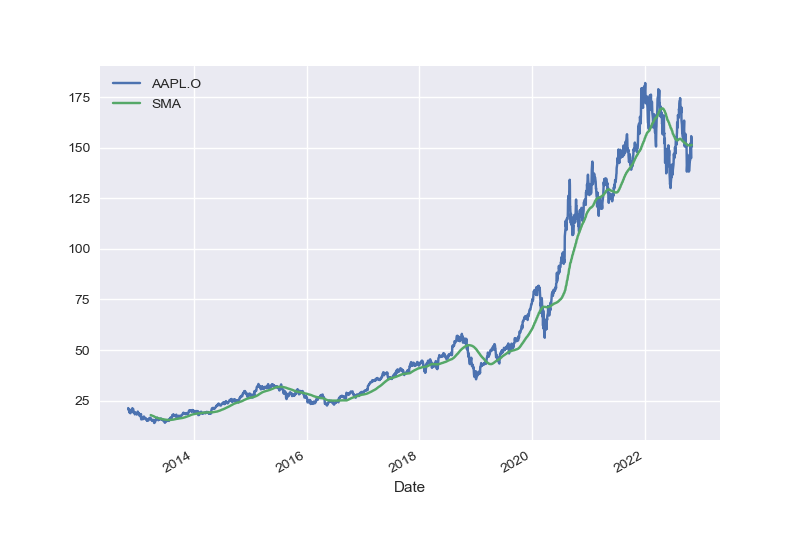
While pandas brings powerful data analysis capabilities, it also comes with most of the advantages of NumPy, such as vectorized operations. The following code creates a small two-dimensional DataFrame object and implements vectorized numerical operations on it.
In [20]: df = pd.DataFrame(np.arange(12).reshape(4, 3))
         df
Out[20]:    0   1   2
         0  0   1   2
         1  3   4   5
         2  6   7   8
         3  9  10  11

In [21]: 2 * df
Out[21]:     0   1   2
         0   0   2   4
         1   6   8  10
         2  12  14  16
         3  18  20  22

In [22]: df ** 3 - df ** 2 + 1.5
Out[22]:        0      1       2
         0    1.5    1.5     5.5
         1   19.5   49.5   101.5
         2  181.5  295.5   449.5
         3  649.5  901.5  1211.5
5. Performance
NumPy and pandas, with their vectorized operations, are already quite fast and in particular faster than pure Python code. However, the vectorization of code is not always the best option or even a feasible option to speed up the execution of Python code. Consider something as simple as the calculation of the sum of all elements of a larger vector. The following Python code implements the summation in pure Python. The memory footprint of the v = range(N) object is negligible with 48 bytes.
In [23]: import sys

In [24]: N = 10_000_000

In [25]: v = range(N)

In [26]: sum(v)
Out[26]: 49999995000000

In [27]: %timeit sum(v)
         103 ms ± 110 µs per loop (mean ± std. dev. of 7 runs, 10 loops each)

In [28]: sys.getsizeof(v)
Out[28]: 48
The implementation of the same task with NumPy in the following code speeds up the code execution considerably. However, the memory footprint increases from 48 bytes to 80 megabytes. In many scenarios, this might be prohibitive.
In [29]: v = np.arange(N)

In [30]: np.sum(v)
Out[30]: 49999995000000

In [31]: %timeit np.sum(v)
         3.79 ms ± 7.63 µs per loop (mean ± std. dev. of 7 runs, 100 loops each)

In [32]: sys.getsizeof(v)
Out[32]: 80000112
One option to increase the execution speed while preserving memory efficiency is the use of dynamic compiling techniques. numba is a Python package that allows the dynamic compilation of pure Python code or code that is a mixture of NumPy and pure Python. The following code first implements the summation as a regular Python function. It then dynamically compiles the function with numba. The performance of the numba compiled version is orders of magnitude faster than the Python version. It also preserves the memory efficiency of the Python version.
In [33]: import numba

In [34]: def sum_py(N):
             s = 0
             for i in range(N):
                 s += i
             return s

In [35]: sum_py(N)
Out[35]: 49999995000000

In [36]: sum_nb = numba.jit(sum_py)

In [37]: sum_nb(N)
Out[37]: 49999995000000

In [38]: %timeit sum_nb(N)
         87.9 ns ± 0.319 ns per loop (mean ± std. dev. of 7 runs, 10,000,000 loops
          each)
Overall, it is safe to say that Python, by applying the right idioms and techniques, is fast enough even for computationally demanding financial algorithms.
6. Input-Output Operations
Execution speed is of the essence in many financial applications. However, reading and writing large data sets often proves to be a bottleneck as well. Fortunately, there are a few options in terms of storage technologies that allow for really fast IO operations.
Consider the following Python code that generates by the use of NumPy a larger sample data set with pseudo-random numbers. The data set is written to disk as a CSV file. This is a relatively slow operation because CSV files are simple text-based files. Similarly, reading the data back from the CSV file is also relatively slow. Nevertheless, CSV is still a standard data exchange format in the financial industry and elsewhere.
In [39]: from numpy.random import default_rng

In [40]: rng = default_rng()

In [41]: N = 10_000_000

In [42]: df = pd.DataFrame(rng.random((N, 2)))

In [43]: fn = '/Users/yves/Temp/data/data.csv'

In [44]: %time df.to_csv(fn)
         CPU times: user 18.6 s, sys: 542 ms, total: 19.1 s
         Wall time: 19.3 s

In [45]: %time new = pd.read_csv(fn, index_col=0, parse_dates=True)
         CPU times: user 5.54 s, sys: 623 ms, total: 6.17 s
         Wall time: 6.28 s
On the other hand, relying on a binary storage technology such as HDF5 (see https://hdfgroup.org) speeds up things considerably. Both, writing the data to disk and reading the data back from disk, are orders of magnitude faster in this case. With technologies such as HDF5, IO operations are often only bound by the speed of the available hardware.
In [46]: fn = '/Users/yves/Temp/data/data.hd5'

In [47]: %time df.to_hdf(fn, 'data')
         CPU times: user 25.1 ms, sys: 83.8 ms, total: 109 ms
         Wall time: 327 ms

In [48]: %time new = pd.read_hdf(fn)
         CPU times: user 18.5 ms, sys: 67.1 ms, total: 85.7 ms
         Wall time: 93.3 ms
If speed is not of the essence, but rather the storage in a more widely used format — such as in an SQL relational database — pandas can also help. The following Python code writes the data set to an SQLite relational database and reads the data back into memory. The speed in this case is much lower as compared to the HDF5-based storage. Overall, the HDF5 option is also the most efficient in terms of file size on disk.
In [49]: import sqlite3 as sq3

In [50]: fn = '/Users/yves/Temp/data/data.sq3'

In [51]: con = sq3.connect(fn)

In [52]: %time df.to_sql('data', con)
         CPU times: user 7.79 s, sys: 1.54 s, total: 9.33 s
         Wall time: 10.1 s

Out[52]: 10000000

In [53]: %time new = pd.read_sql('SELECT * FROM data', con)
         CPU times: user 6.08 s, sys: 3.59 s, total: 9.67 s
         Wall time: 11.4 s

In [54]: ls -n /Users/yves/Temp/data
         total 2272264
         -rw-r--r--  1 501  20  464285269 Dec 19 14:30 data.csv
         -rw-r--r--  1 501  20  240007240 Dec 19 14:30 data.hd5
         -rw-r--r--  1 501  20  443166720 Dec 19 14:30 data.sq3

In [55]: rm /Users/yves/Temp/data/data.*
7. Get Your Next Belt in Python
If you are interested in entering the financial industry or accelerating your career in it, there is hardly any better option than to learn Python programming and advance your level from either white to green belt or from green belt to brown belt. Like English as a spoken language and mathematics as a symbolic language, Python can be considered universal in its reach, scope, and applicability. This not only holds true for finance but for other domains as well. It also holds true for such fundamental technologies as machine learning and artificial intelligence. Python is indeed everywhere these days and picking it up might be one of the best options to turbo-charge your career.