Reinforcement Learning for Finance

Copyright

This document as well as the accompanying code, Jupyter Notebooks, and other materials on the Quant Platform (http://pqp.io) and Github are copyrighted and only intended for personal use. Any kind of sharing, distribution, duplication, commercial use, etc. without written permission by Dr. Yves J. Hilpisch is prohibited.

The contents, Python code, Jupyter Notebooks, and other materials of this book come without warranties or representations, to the extent permitted by applicable law.

Notice that this document is work in progress and that substantial additions, changes, updates, etc. will take place over time. It is advised to regularly check for new versions of the document.

Preface

Tell me and I forget. Teach me and I remember. Involve me and I learn.

— Benjamin Franklin

Why this Book?

Reinforcement learning (RL) has enabled a number of breakthroughs in artificial intelligence. One of the key algorithms in RL is deep Q-learning (DQL) that can be applied to a large number of dynamic decision problems. Popular examples are arcade games and board games, such as Go, for which RL and DQL algorithms have achieved superhuman performance in many instances. This has often happened despite the beliefs of experts that such feats would be impossible for decades to come.

Finance is a discipline with a strong connection between theory and practice. Theoretical advancements often find their way quickly into the applied domain. Many problems in finance are dynamic decision problems, such as the optimal allocation of assets over time. Therefore it is, on the one hand, theoretically interesting to apply DQL to financial problems. On the other hand, it is also in general quite easy and straightforward to apply such algorithms — usually after some thorough testing — in the financial markets.

In recent years, financial research has seen a strong growth in publications related to RL, DQL, and related methods applied to finance. However, there is hardly any resource in book form — beyond the purely theoretical ones — for those who are looking for an applied introduction to this exciting field. This book closes the gap in that it provides the required background in a concise fashion and otherwise focuses on the implementation of the algorithms in the form of self-contained Python code and the application to important financial problems.

Target Audience

This book is intended as a concise, Python-based introduction to the major ideas and elements of RL and DQL as applied to finance. It should be useful to both students and academics as well as to practitioners in search of alternatives to existing financial theories and algorithms. The book expects basic knowledge of the Python programming language, object-oriented programming, and the major Python packages used in data science and machine learning, such as NumPy, pandas, matplotlib, scikit-learn, and TensorFlow.

Overview of the Book

The book consists of the following chapters:

Learning through Interaction: The first chapter focuses on learning through interaction with four major examples: probability matching, Bayesian updating, reinforcement learning (RL), and deep-Q-learning (DQL).
Deep Q-Learning: The second chapter introduces concepts from dynamic programming (DP) and discusses DQL as an approach to approximate solutions to DP problems. The major theme is the derivation of optimal policies to maximize a given objective function through taking a sequence of actions and updating the optimal policy iteratively. DQL is illustrated on the basis of a DQL agent that learns to play the CartPole game from the gymnasium Python package.
Financial Q-Learning: The third chapter develops a first finance environment that allows the DQL agent from Deep Q-Learning to learn a financial prediction game. Although the environment formally replicates the API of the CartPole it misses yet some important characteristics to apply RL successfully.
Simulated Data: The fourth chapter is about data augmentation based on Monte Carlo simulation approaches and discusses the addition of noise to historical data and the simulation of stochastic processes.
Generated Data: The fifth chapter introduces generative adversarial networks (GANs) to synthetically generate time series data that has similar statistical characteristics as historical time series data on which a GAN was trained on.
Algorithmic Trading: Building on the example from Financial Q-Learning, this chapter applies DQL to the problem of algorithmic trading based on the prediction of the next price movement’s direction.
Dynamic Hedging: The seventh chapter is about the learning of optimal dynamic hedging strategies for an option with European exercise in the Black-Scholes-Merton (1973) model. In other words, delta hedging or dynamic replication of the option is the goal.
Dynamic Asset Allocation: This chapter applies DQL to three canonical examples in asset management: one risky asset and one risk-less asset, two risky assets, and three risky assets. The problem is to dynamically allocate funds to the available assets to maximize a profit target or a risk-adjusted return (Sharpe ratio).
Optimal Execution: The tenth chapter is about the optimal liquidation of a large position in a stock. Given a certain risk aversion, the total execution costs are to be minimized. This use case differs from the others in that all actions are tightly connected with each other through an additional constraint. The chapter also introduces an additional RL algorithm in the form of an actor-critic implementation.
Concluding Remarks: The final chapter of the book provides some concluding remarks and sketches out how the examples presented in the book can be improved upon.

The Basics

The first part of the book covers the basics of reinforcement learning and provides background information. It consists of three chapters:

Learning through Interaction focuses on learning through interaction with four major examples: probability matching, Bayesian updating, reinforcement learning (RL), and deep-Q-learning (DQL).
Deep Q-Learning introduces concepts from dynamic programming (DP) and discusses DQL as an approach to approximate solutions to DP problems. The major theme is the derivation of optimal policies to maximize a given objective function through taking a sequence of actions and updating the optimal policy iteratively. DQL is illustrated based on the CartPole game from the gymnasium Python package.
Financial Q-Learning develops a first finance environment that allows the DQL agent from Deep Q-Learning to learn a financial prediction game. Although the environment formally replicates the application programming interface (API) of the CartPole, it misses yet some important characteristics to apply RL successfully.

1. Learning through Interaction

The idea that we learn by interacting with our environment is probably the first to occur to us when we think about the nature of learning.

— Sutton and Barto (2018)

For human beings and animals alike, learning is almost as fundamental as breathing. It is something that happens continuously and most often unconsciously. There are different forms of learning. The one most important to the topics covered in this book is based on interacting with an environment.

Interaction with an environment provides the learner — or agent henceforth — with feedback that can be used to update their knowledge or to refine a skill. In this book, we are mostly interested in learning quantifiable facts about an environment, such as the odds of winning a bet or the reward that an action yields.

Bayesian Learning discusses Bayesian learning as an example of learning through interaction. Reinforcement Learning presents breakthroughs in artificial intelligence that were made possible through reinforcement learning. It also describes the major building blocks of reinforcement learning. Deep Q-Learning explains the two major characteristics of deep Q-learning which is the most important algorithm for the remainder of the book.

1.1. Bayesian Learning

Two simple examples can illustrate learning by interacting with an environment: tossing a biased coin and rolling a biased die. The examples are based on the idea that an agent betting repeatedly on the outcome of a biased gamble — and remembering all outcomes — can learn bet-by-bet about a gamble’s bias and therewith about the optimal policy for betting. The idea, in that sense, makes use of Bayesian updating. Bayes theorem and Bayesian updating date back to the 18th century (see Bayes and Price (1763)). A modern and Python-based discussion of Bayesian statistics is found in Downey (2021).

1.1.1. Tossing a Biased Coin

Assume the simple game of betting on the outcome of tossing a biased coin. As a benchmark, consider the special case of an unbiased coin first. Agents are allowed to bet for free on the outcome of the coin tosses. An agent might, for example, bet randomly on either heads or tails. If the agent wins, the reward is 1 USD and nothing otherwise. The agent’s goal is to maximize the total reward. The following Python code simulates several sequences of 100 bets each:

In [1]: import numpy as np
        from numpy.random import default_rng
        rng = default_rng(seed=100)

In [2]: ssp = [1, 0]  (1)

In [3]: asp = [1, 0]  (2)

In [4]: def epoch():
            tr = 0
            for _ in range(100):
                a = rng.choice(asp)  (3)
                s = rng.choice(ssp)  (4)
                if a == s:
                    tr += 1  (5)
            return tr

In [5]: rl = np.array([epoch() for _ in range(250)])  (6)
        rl[:10]
Out[5]: array([56, 47, 48, 55, 55, 51, 54, 43, 55, 40])

In [6]: rl.mean()  (7)
Out[6]: 49.968

1	The state space, `1` for heads and `0` for tails.
2	The action space, `1` for a bet on heads and `0` for one on tails.
3	The random bet.
4	The random coin toss.
5	The reward for a winning bet.
6	The simulation of multiple sequences of bets.
7	The average total reward.

The average total reward in this benchmark case is close to 50. The same result might be achieved by solely betting on either heads or tails.

Assume now that the coin is biased in a way that heads prevails in 80% of the coin tosses. Betting solely on heads would yield an average total reward of about 80 for 100 bets. Betting solely on tails would yield an average total reward of about 20. But what about the random betting strategy? The following Python code simulates this case:

In [7]: ssp = [1, 1, 1, 1, 0]  (1)

In [8]: asp = [1, 0]  (2)

In [9]: def epoch():
            tr = 0
            for _ in range(100):
                a = rng.choice(asp)
                s = rng.choice(ssp)
                if a == s:
                    tr += 1
            return tr

In [10]: rl = np.array([epoch() for _ in range(250)])
         rl[:10]
Out[10]: array([53, 56, 40, 55, 53, 49, 43, 45, 50, 51])

In [11]: rl.mean()
Out[11]: 49.924

1	The biased state space.
2	The same action space as before.

Although the coin is now highly biased the average total reward of the random betting strategy is about the same as in the benchmark case. This might sound counterintuitive. However, the expected win rate is given by $0.8 \cdot 0.5 + 0.2 \cdot 0.5 = 0.5$. In words, when betting on heads the win rate is 80% and when betting on tails it is 20%. Together, the total reward is as before on average. As a consequence, without learning, the agent is not able to capitalize on the bias.

A learning agent on the other hand can gain an edge by basing the betting strategy on the previous outcomes they observe. To this end, it is already enough to record all observed outcomes and to choose randomly from the set of all previous outcomes. In this case, the bias is reflected in the number of times the agent randomly bets on heads as compared to tails. The Python code that follows illustrates this simple learning strategy:

In [12]: ssp = [1, 1, 1, 1, 0]

In [13]: def epoch(n):
             tr = 0
             asp = [0, 1]  (1)
             for _ in range(n):
                 a = rng.choice(asp)
                 s = rng.choice(ssp)
                 if a == s:
                     tr += 1
                 asp.append(s)  (2)
             return tr

In [14]: rl = np.array([epoch(100) for _ in range(250)])
         rl[:10]
Out[14]: array([71, 65, 67, 69, 68, 72, 68, 68, 77, 73])

In [15]: rl.mean()
Out[15]: 66.78

1	The initial action space.
2	The update of the action space with the observed outcome.

With remembering and learning, the agent achieves an average total reward of about 66.8 — a significant improvement over the random strategy without learning. This is close to the expected value of $(0.8^2 + 0.2^2) \cdot 100 = 68$.

This strategy, while not optimal, is regularly observed in experiments involving human beings — and maybe somewhat surprisingly in animals as well. It is called probability matching.

Probability Matching

Koehler and James (2014) report results from studies analyzing probability matching, utility maximization, and other types of decision strategies.^[1] The studies include a total of 1,557 university students.^[2] The researchers find that probability matching is the most frequent strategy chosen or a close second to the utility maximizing strategy.

The researchers also find that the utility maximizing strategy is chosen in general by the “most cognitively able participants”. They approximate cognitive ability through Scholastic Aptitude Test (SAT) scores, Mathematics Experience Composite scores, and the Number of University Statistics courses taken.

As is often the case in decision-making, human beings might need formal training and experience to overcome urges and behaviors that feel natural to achieve optimal results.

On the other hand, the agent can do better by simply betting on the most likely outcome as derived from past results. The following Python code implements this strategy.

In [16]: from collections import Counter

In [17]: ssp = [1, 1, 1, 1, 0]

In [18]: def epoch(n):
             tr = 0
             asp = [0, 1]  (1)
             for _ in range(n):
                 c = Counter(asp)  (2)
                 a = c.most_common()[0][0]  (3)
                 s = rng.choice(ssp)
                 if a == s:
                     tr += 1
                 asp.append(s)  (4)
             return tr

In [19]: rl = np.array([epoch(100) for _ in range(250)])
         rl[:10]
Out[19]: array([81, 70, 74, 77, 82, 74, 81, 80, 77, 78])

In [20]: rl.mean()
Out[20]: 78.828

1	The initial action space.
2	The frequencies of the action space elements.
3	The action is chosen with the highest frequency.
4	The update of the action space with the observed outcome.

In this case, the gambler achieves an average total reward of 78.5 which is close to the theoretical optimum of 80. In this context, this strategy seems to be the optimal one.

1.1.2. Rolling a Biased Die

As another example, consider a biased die. For this die, the probability for the outcome “4” shall be five times as likely as for any other number of the six-sided die. The following Python code simulates sequences of 600 bets on the outcome of the die, where a correct bet is rewarded with 1 USD and nothing otherwise.

In [21]: ssp = [1, 2, 3, 4, 4, 4, 4, 4, 5, 6]  (1)

In [22]: asp = [1, 2, 3, 4, 5, 6]  (2)

In [23]: def epoch():
             tr = 0
             for _ in range(600):
                 a = rng.choice(asp)
                 s = rng.choice(ssp)
                 if a == s:
                     tr += 1
             return tr

In [24]: rl = np.array([epoch() for _ in range(250)])
         rl[:10]
Out[24]: array([ 92,  96, 106,  99,  96, 107, 101, 106,  92, 117])

In [25]: rl.mean()
Out[25]: 101.22

1	The biased state space.
2	The uninformed action space.

Without learning, the random betting strategy yields an average total reward of about 100. With perfect information about the biased die, the agent could expect an average total reward of about 300 because it would win about 50% of the 600 bets.

With probability matching, the agent will not achieve a perfect outcome — as was the case with the biased coin. However, the agent can improve the average total reward by more than 75% as the following Python code shows:

In [26]: def epoch():
             tr = 0
             asp = [1, 2, 3, 4, 5, 6]  (1)
             for _ in range(600):
                 a = rng.choice(asp)
                 s = rng.choice(ssp)
                 if a == s:
                     tr += 1
                 asp.append(s)  (2)
             return tr

In [27]: rl = np.array([epoch() for _ in range(250)])
         rl[:10]
Out[27]: array([182, 174, 162, 157, 184, 167, 190, 208, 171, 153])

In [28]: rl.mean()
Out[28]: 176.296

1	The initial action space.
2	The update of the action space.

The average total reward increases to about 177, which is not that far from the expected value of that strategy of $(0.5^2 + 0.1^2 \cdot 5) \cdot 600 = 180$.

As with the biased coin tossing game, the agent again can do better by simply choosing the action with the highest frequency in the updated action space, as the following Python code confirms. The average total reward of 299 is pretty close to the theoretical maximum of 300:

In [29]: def epoch():
             tr = 0
             asp = [1, 2, 3, 4, 5, 6]  (1)
             for _ in range(600):
                 c = Counter(asp)  (2)
                 a = c.most_common()[0][0]  (3)
                 s = rng.choice(ssp)
                 if a == s:
                     tr += 1
                 asp.append(s)  (4)
             return tr

In [30]: rl = np.array([epoch() for _ in range(250)])
         rl[:10]
Out[30]: array([305, 288, 312, 306, 318, 302, 304, 311, 313, 281])

In [31]: rl.mean()
Out[31]: 297.204

1	The initial action space.
2	The frequencies of the action space elements.
3	The action is chosen with the highest frequency.
4	The update of the action space with the observed outcome.

1.1.3. Bayesian Updating

The Python code and simulation approach in the previous sub-sections make for a simple way to implement the learning of an agent through playing a potentially biased game. In other words, by interacting with the betting environment, the agent can update their estimates for the relevant probabilities.

The procedure can therefore be interpreted as Bayesian updating of probabilities — to find out, for example, the bias of a coin.^[3] The following discussion illustrates this insight based on the coin-tossing game.

Assume that the probability for heads (h) is $P(h) = \alpha$ and that the probability for tails (t) accordingly is $P(t) = 1 - \alpha$. The coin flips are assumed to be identically and independently distributed (i.i.d) according to the binomial distribution. Assume that an experiment yields $f_h$ times heads and $f_t$ times tails. Furthermore, assume that the binomial coefficient is given by:

\[B = \binom{f_h + f_t}{f_h}\]

In that case, we get $P(E | \alpha) = B \cdot \alpha^{f_h} \cdot (1 - \alpha)^{f_t}$ as the probability that the experiment yields the assumed observations. $E$ represents the event that $f_h$ times heads and $f_t$ times tails is observed.

One approach to deriving an appropriate value for $\alpha$ given the results from the experiment is maximum likelihood estimation (MLE). The goal of MLE is to find a value $\alpha$ that maximizes $P(E | \alpha)$. The problem to solve as follows:

\[\begin{array}{} \alpha^{MLE} &=& \underset{\alpha}{\arg\!\max} P(E | \alpha) \\ &=& \underset{\alpha}{\arg\!\max} \ln P(E | \alpha) \\ &=& \underset{\alpha}{\arg\!\max} \ln (B \cdot \alpha^{f_h} \cdot (1 - \alpha)^{f_t}) \\ &=& \underset{\alpha}{\arg\!\max} \ln B + f_h \ln \alpha + f_t \ln(1 - \alpha) \end{array}\]

With this, one derives the optimal estimator by taking the first derivative with respect to $\alpha$ and setting it equal to zero:

\[\begin{array}{} \frac{d}{d\alpha} P(E | \alpha) &=& 0 \\ f_h \frac{d}{d\alpha} \ln \alpha + f_t \frac{d}{d\alpha} \ln(1 - \alpha) &=& 0 \\ \frac{f_h}{\alpha} - \frac{f_t}{1-\alpha} &=& 0 \end{array}\]

Simple manipulations yield the following maximum likelihood estimator:

\[\alpha^{MLE} = \frac{f_h}{f_h + f_t}\]

$\alpha^{MLE}$ is the frequency of heads over the total number of flips in the experiment. This is what has been learned flip-by-flip through the simulation approach, that is, through an agent betting on the outcomes of coin flips one after the other and remembering previous outcomes.

In other words, the agent has implemented Bayesian updating incrementally and bet-by-bet to arrive, after enough bets, to a numerical estimator $\hat{\alpha}$ close to $\alpha^{MLE}$, that is, $\hat{\alpha} \approx \alpha^{MLE}$.

1.2. Reinforcement Learning

Reinforcement learning (RL) is a type of machine learning (ML) algorithm that relies on the interaction of an agent with an environment. This aspect is similar to the agent playing a potentially biased game and learning about relevant probabilities. However, RL algorithms are more general and capable in that an agent can learn from high-dimensional input to accomplish complex tasks.

While the mode of learning, interaction or trial and error, differs from other ML methods, the goals are nevertheless the same. Mitchell (1997) defines ML as follows:

A computer program is said to learn from experience $E$ with respect to some class of tasks $T$ and performance measure $P$, if its performance at tasks in $T$, as measured by $P$, improves with experience $E$.

— Mitchell (1997)

This section provides some general background to RL while the next chapter introduces more technical details. Sutton and Barto (2018) provide a comprehensive overview of RL approaches and algorithms. On a high level, they describe RL as follows:

Reinforcement learning is about learning from interaction how to behave in order to achieve a goal. The reinforcement learning agent and its environment interact over a sequence of discrete time steps.

Reinforcement Learning

Most books on ML focus on supervised and unsupervised learning algorithms, but RL is the learning approach that comes closest to how human beings and animals learn. Namely, through repeated interaction with their environment and receiving positive (reinforcing) or negative (punishing) feedback. Such a sequential approach is much closer to human learning than the simultaneous learning from a generally very large number of labeled or unlabeled examples.

1.2.1. Major Breakthroughs

In artificial intelligence (AI) research and practice, two types of algorithms have seen a meteoric rise over the last ten years: deep neural networks (DNNs) and reinforcement learning (RL).^[4] While DNNs have seen their own success stories in many different application areas, they also play an integral role in modern RL algorithms, such as Q-learning.^[5]

The book by Gerrish (2018) recounts several major success stories — and sometimes also failures — of AI over recent decades. In almost all of them, DNNs play a central role and RL algorithms sometimes are also a core part of the story. Among those successes are playing Atari 2600 games, chess, and Go on superhuman levels. These are discussed in what follows.

Concerning RL, and Q-learning in particular, the company DeepMind has achieved several noteworthy breakthroughs. In Mnih et al. (2013) and Mnih et al. (2015), the company reports how a so-called deep Q-learning (DQL) agent can learn to play Atari 2600 console^[6] games on a superhuman level through interacting with a game-playing API. Bellemare et al. (2013) provide an overview of this popular API for the training of RL agents.

While mastering Atari games is impressive for an RL agent, and was celebrated by the AI researcher and retro gamer communities alike, the breakthrough concerning popular board games, such as Go and chess, gained the highest public attention and admiration.

In 2014, researcher and philosopher Nick Bostrom predicted in his popular book Superintelligence that it might take another 10 years for AI researchers to come up with an AI agent that plays the game of Go on a superhuman level:

Go-playing programs have been improving at a rate of about 1 dan/year in recent years. If this rate of improvement continues, they might beat the human world champion in about a decade.

However, DeepMind researchers were able to successfully leverage the DQL techniques developed for playing Atari games and to come up with a DQL agent, called AlphaGo, that first beat the European champion in Go in 2015 and later in early 2016 even the world champion.^[7] The details are documented in Silver et al. (2017). They summarize:

A long-standing goal of artificial intelligence is an algorithm that learns, tabula rasa, superhuman proficiency in challenging domains. Recently, AlphaGo became the first program to defeat a world champion in the game of Go. The tree search in AlphaGo evaluated positions and selected moves using deep neural networks. These neural networks were trained by supervised learning from human expert moves, and by reinforcement learning from self-play.

DeepMind was able to generalize the approach of AlphaGo, which primarily relies on DQL agents playing a large number of games against themselves (“self-playing”), to the board games of chess and shogi. DeepMind calls this generalized agent AlphaZero. What is most impressive about AlphaZero is that only a few hours of self-playing chess for training are enough to reach not only a superhuman level but also a level well above any other computer engine, such as Stockfish. The paper by Silver et al. (2018) provides the details and summarizes:

In this paper, we generalize this approach into a single AlphaZero algorithm that can achieve superhuman performance in many challenging games. Starting from random play and given no domain knowledge except the game rules, AlphaZero convincingly defeated a world champion program in the games of chess and shogi (Japanese chess), as well as Go.

The paper also provides the following training times:

Training lasted for approximately 9 hours in chess, 12 hours in shogi, and 13 days in Go …

The dominance of AlphaZero over Stockfish in chess is not only remarkable given the short training time. It is also remarkable because AlphaZero only evaluates a much lower number of positions per second:

AlphaZero searches just 60,000 positions per second in chess and shogi, compared with 60 million for Stockfish …

One is inclined to attribute this to some form of acquired tactical and strategic intelligence on the side of AlphaZero as compared to predominantly brute force computation on the side of Stockfish.

Reinforcement and Deep Learning

The breakthroughs in AI outlined in this sub-section rely on a combination of RL and DL. While DL can be applied in many scenarios, such as standard supervised and unsupervised learning situations, without RL, RL is in general today exclusively applied with the help of DL and DNNs.

1.2.2. Major Building Blocks

It is not that simple to exactly pin down why DQL algorithms are so successful in many domains that were obviously so hard to crack by computer scientists and AI researchers for decades. However, it is relatively straightforward to describe the major building blocks of an RL and DQL algorithm.

It generally starts with an environment. This can be an API to play Atari games, an environment to play chess, or an environment for navigating a map indoors or outdoors. Nowadays, there are many such environments available to get started with RL efficiently. One of the most popular ones is the Gymnasium environment.^[8] On the Github page you read:

Gymnasium is an open source Python library for developing and comparing reinforcement learning algorithms by providing a standard API to communicate between learning algorithms and environments, as well as a standard set of environments compliant with that API.

At any given point, an environment is characterized by a state. The state summarizes all the relevant, and sometimes also irrelevant, information for an agent to receive as input when interacting with an environment. Concerning chess, a board position with all relevant pieces represents such a state. Sometimes additional input is required like, for example, whether castling has happened or not. For an Atari game, the pixels of the screen and the current score could represent the state of the environment.

The agent in this context subsumes all elements of the RL algorithm that interact with the environment and that learn from these interactions. In an Atari games context, the agent might represent a player playing the game. In the context of chess, it can be either the player playing the white or black pieces.

An agent can choose one action from an often finite set of allowed actions. In an Atari game, movements to the left or right might be allowed actions. In chess, the rule set specifies both the number of allowed actions and their types.

Given the action of an agent, the state of the environment is updated. One such update is generally called a step. The concept of a step is general enough to encompass both heterogeneous and homogeneous time intervals between two steps. Whereas in Atari games, for example, real-time interaction with the game environment is simulated by rather short, homogeneous time intervals (“game clock”), chess players have quite some flexibility with regard to how long it takes them to make the next move (take the next action).

Depending on the action an agent chooses, a reward or penalty is awarded. For an Atari game, points are a typical reward. In chess, it is often a bit more subtle in that an evaluation of the current board position must take place. Improvements in the evaluation then represent a reward while a worsening of the evaluation represents a penalty.

In RL, an agent is assumed to maximize an objective function. For Atari games, this can simply be the score achieved, that is, the sum of points collected during gameplay. In other words, it is a hunt for new “high scores”. In playing chess, it is to set the opponent checkmate as represented by, say, an infinite evaluation score of the board position.

The policy defines which action an agent takes given a certain state of the environment. This is done by assigning values — technically, floating point numbers — to all possible combinations of states and actions. An optimal action is then chosen by looking up the highest value possible for the current state and the set of possible actions. Given a certain state in an Atari game, represented by all the pixels that make up the current scene, the policy might specify that the agent chooses “move right” as the optimal action. In chess, given a specific board position, the policy might specify to move the white king from c1 to b1.

An episode is a collection of steps from the initial state of the environment until success is achieved or failure is observed. In an Atari game, this means from the start of the game until the agent has lost all “lives” — or has maybe achieved a final goal of the game. In chess, an episode represents a full game until a win, loss, or draw.

In summary, RL algorithms are characterized by the following building blocks:

Environment
State
Agent
Action
Step
Reward
Objective
Policy
Episode

Modeling Environments

The famous quote “Things should be as simple as possible, but no simpler”, usually attributed to Albert Einstein, can serve as a guideline for the design of environments and their APIs for reinforcement learning. Like in the context of a scientific model, an environment should capture all relevant aspects of the phenomena to be covered by it and dismiss those that are irrelevant. Sometimes, tremendous simplifications can be made based on this approach. At other times, an environment must represent the complete problem at hand. For example, when playing chess the complete board position with all the pieces is relevant.

1.3. Deep Q-Learning

What characterizes so-called deep Q-learning (DQL) algorithms? To begin with, QL is a special form of RL. In that sense, all the major building blocks of RL algorithms apply to QL algorithms as well. There are two specific characteristics of DQL algorithms.

First, DQL algorithms evaluate both the immediate reward of an agent’s action and the delayed reward of the action. The delayed reward is estimated through an evaluation of the state that unfolds when the action is taken. The evaluation of the unfolding state is done under the assumption that all actions going forward are chosen optimally.

In chess, it is obvious that it is by far not sufficient to evaluate the very next move. It is rather necessary to look a few moves ahead and to evaluate different alternatives that can ensue. A chess novice has a hard time, in general, looking just two or three moves ahead. A chess grandmaster on the other hand can look as far as 20 to 30 moves ahead, as some argue.^[9]

Second, DQL algorithms use DNNs to approximate, learn, and update the optimal policy. For most interesting environments in RL, the mapping of states and possible actions to values is too complex to be modeled explicitly, say, through a table or a mathematical function. DNNs are known to have excellent approximation capabilities and provide all the flexibility needed to accommodate almost any type of state that an environment might communicate to the DQL agent.

Considering again chess as an example, it is estimated that there are more than $10^{100}$ possible moves, with illegal moves included. This compares to $10^{80}$ as an estimate for the number of atoms in the universe. With legal moves only, there are about $10^{40}$ possible moves, which is still a pretty large number:

In [32]: cm = 10 ** 40
         print(f'{cm:,}')
         10,000,000,000,000,000,000,000,000,000,000,000,000,000

This shows that only an approximation of the optimal policy is feasible in almost all interesting RL cases.

1.4. Conclusions

This chapter focuses on learning through interaction with an environment. It is a natural phenomenon, observed in human beings and animals alike. Simple examples show how an agent can learn probabilities through repeatedly betting on the outcome of a gamble and thereby implementing Bayesian updating. For this book, RL algorithms are the most important ones. Breakthroughs related to RL and the building blocks of RL are discussed. DQL, as a special RL algorithm, is characterized by taking into account not only immediate rewards but also delayed rewards from taking an action. In addition, the optimal policy is generally approximated by DNNs. Later chapters cover the DQL algorithm in much more detail and use it extensively.

1.5. References

Articles and books cited in this chapter:

Bayes, Thomas and Richard Price (1763): “An Essay towards Solving a Problem in the Doctrine of Chances. By the Late Rev. Mr. Bayes, F.R.S. Communicated by Mr. Price, in a Letter to John Canton, A.M. F.R.S” Philosophical Transactions of the Royal Society of London, Vol. 53, 370–418.
Bellemare, Marc et al. (2013): “The Arcade Learning Environment: An Evaluation Platform for General Agents.” Journal of Artificial Intelligence Research, Vol. 47, 253–279.
Bostrom, Nick (2014): Superintelligence—Paths, Dangers, Strategies. Oxford University Press, Oxford.
Downey, Allen (2021): Think Bayes. 2nd. ed., O’Reilly Media, Sebastopol.
Gerrish, Sean (2018): How Smart Machines Think. MIT Press, Cambridge.
Goodfellow, Ian, Yoshua Bengio, and Aaron Courville (2016): Deep Learning. MIT Press, Cambridge, http://deeplearningbook.org.
Hanel, Paul, Katia Vione (2016): “Do Student Samples Provide an Accurate Estimate of the General Public?” PLoS ONE, Vol. 11, No. 12.
Mitchell, Tom (1997): Machine Learning. McGraw-Hill, New York.
Mnih, Volodymyr et al. (2013): “Playing Atari with Deep Reinforcement Learning” https://doi.org/10.48550/arXiv.1312.5602.
Mnih, Volodymyr et al. (2015): “Human-Level Control through Deep Reinforcement Learning” Nature, Vol. 518, 529–533.
Rachev, Svetlozar et al. (2008): Bayesian Methods in Finance. John Wiley & Sons, Hoboken.
Silver, David et al. (2017): “Mastering the Game of Go without Human Knowledge.” Nature, Vol. 550, 354–359.
Silver, David et al. (2018): “A General Reinforcement Learning Algorithm that Masters Chess, Shogi and Go through Self-Play”. Science, Vol. 362, Issue 6419, 1140-1144.
Sutton, Richard and Andrew Barto (2018): Reinforcement Learning: An Introduction. 2nd ed., The MIT Press, Cambridge and London.
Watkins, Christopher (1989): Learning from Delayed Rewards. Ph.D. thesis, University of Cambridge.
Watkins, Christopher and Peter Dayan (1992): “Q-Learning.” Machine Learning, Vol. 8, 279-282.
West, Richard and Keith Stanovich (2003): “Is Probability Matching Smart? Associations Between Probabilistic Choices and Cognitive Ability.” Memory & Cognition, Vol. 31, No. 2, 243-251.

2. Deep Q-Learning

Like a human, our agents learn for themselves to achieve successful strategies that lead to the greatest long-term rewards. This paradigm of learning by trial-and-error, solely from rewards or punishments, is known as reinforcement learning (RL).^[10]

— DeepMind (2016)

The previous chapter introduces deep Q-learning (DQL) as a major algorithm in artificial intelligence (AI) to learn through interaction with an environment. This chapter provides some more details about the DQL algorithm. It uses the CartPole environment from the gymnasium Python package to illustrate the API-based interaction with gaming environments. It also implements a DQL agent as a self-contained Python class that serves as a blueprint for later DQL agents applied to financial environments.

However, before the focus is turned on DQL the chapter discusses general decision problems in economics and finance. Dynamic programming is introduced as a solution mechanism for dynamic decision problems. This provides the background for the application of DQL algorithms because they can be considered to lead to approximate solutions to dynamic programming problems.

Decision Problems classifies decision problems in economics and finance according to different characteristics. Dynamic Programming focuses on a special type of decision problem, so-called finite horizon Markovian dynamic programming problems. Q-Learning outlines the major elements of Q-learning and explains the role of deep neural networks in this context. Finally, CartPole as an Example illustrates a DQL setup by the use of the CartPole game API and a DQL agent implemented as a Python class.

2.1. Decision Problems

In economics and finance, optimization and associated techniques play a central role. One could almost say that finance is nothing else than the systematic application of optimization techniques to problems arising in a financial context. Different types of optimization problems can be distinguished in finance. The major differentiating criteria as follows:

Discrete vs. continuous action space: The quantities or actions to be chosen through optimization can be from a set of finite, discrete options (optimal choice) or from a set of infinite, continuous options (optimal control).
Static vs. dynamic problems: Some problems are one-off optimization problems — these are generally called static problems. Other problems are characterized by a typically large number of sequential and connected optimization problems over time — these are called dynamic problems.
Finite vs. infinite horizon: Dynamic optimization problems can have a finite or infinite horizon. Playing a game of chess generally has a finite horizon.^[11] Estate planning for multiple generations of a family can be seen as a decision problem with an infinite horizon. Climate policy might be another one.
Discrete vs. continuous time: Some dynamic problems only require discrete decisions and optimizations at different points in time. Chess playing is again a good example. Other dynamic problems require continuous decisions and optimizations. Driving a car or flying an airplane are examples for when a driver or pilot needs to continuously make sure that appropriate decisions are made.

Given the examples discussed in Learning through Interaction, betting on the outcome of a biased coin is a static problem with discrete action space. Although such a bet can be repeated multiple times, the optimal betting strategy is independent of the previous bet as well as of the next bet. On the other hand, playing a game of chess is a dynamic problem — with a finite horizon — because a player needs to make a sequence of optimal decisions that are all dependent on each other. The current board position depends on the player’s (and the opponent’s) previous moves. The future move options (action space) depend on the current move the player chooses.

In summary, because the action space is finite in both cases, coin betting is a discrete, static optimization problem, whereas playing chess is a discrete, dynamic optimization problem with finite horizon.

2.2. Dynamic Programming

An important type of dynamic optimization problem is the finite horizon Markovian dynamic programming problem (FHMDP). An FHMDP can formally be described by the following tuple^[12]:

\[\{S, A, T, (r_t, f_t, \Phi_t)_{t=0}^T\}\]

$S$ is the state space of the problem with generic element $s$. $A$ is the action space of the problem with generic element $a$. $T$ is a positive integer and represents the finite horizon of the problem.

For each point in time, at which an action is to be chosen, $t \in \{0, 1, \dots , T\}$, there are two relevant functions and one relevant correspondence. The reward function maps a state and an action to a real-valued reward. If an agent at time $t$ chooses action $a_t$ in state $s_t$ they receive a reward of $r_t$:

\[r_t: S \times A \rightarrow \mathbb{R}\]

The transition function maps a state and an action to another state. This function models the step from state $s_t$ to state $s_{t+1}$ when action $a_t$ is taken:

\[f_t: S \times A \rightarrow S\]

Finally, the feasible action correspondence maps states to feasible actions. Given a state $s_t$, the correspondence defines all feasible actions $\{a_t^1, a_t^2, \dots \}$ for that state:

\[\Phi_t: S \rightarrow P(A)\]

The objective of an agent is to choose a plan for taking actions at each point in time to maximize the sum of the per-period rewards over the horizon of the model. In other words, an agent needs to solve the following optimization problem:

\[\underset{ a_t, t \in \{0, 1, \dots , T\} }{ \max }\sum_{t=1}^T r_t(s_t,a_t)\]

subject to

\[\begin{cases}{} s_0 &=& s \in S \\ s_t &=& f_{t-1}(s_{t-1}, a_{t-1}), t=1, \dots, T \\ a_t &\in& \Phi_t(s_t), t=1, \dots, T \end{cases}\]

What does Markovian mean in this context? It means that the transition function only depends on the current state and the current action taken and not on the full history of all states and actions. Formally, the following equality holds.

\[s_t = f_{t-1}(s_{t-1}, a_{t-1}) = f_{t-1}(s_{t-1},s_{t-2},\dots; a_{t-1}, a_{t-2}, \dots)\]

In this context, one also needs to distinguish between FHMDP problems for which the transition function is deterministic or stochastic. For chess, it is clear that the transition function is deterministic. On the other hand, typical computer games and all games offered in casinos generally have stochastic elements and as a consequence stochastic transition functions. If the transition function is stochastic, one usually speaks of stochastic dynamic programming.

A Markovian policy $\sigma$ is a contingency plan that specifies which action $a$ is to be taken if state $s$ is observed. For an FHMDP, this implies $\sigma: S \rightarrow A$ with $\sigma_t(s_t) \in \Phi_t(s_t)$. This gives the set of all feasible policies, $\sigma \in \Sigma$.

The total reward of a feasible policy $\sigma$ is denoted by

\[W(s_0, \sigma) = \sum_{t=1}^T r_t(s_t, \sigma_t)\]

The value function $V: S \rightarrow \mathbb{R}$ is then defined by the supremum of the total reward over all feasible policies:

\[V(s_0) = \sup_{\sigma \in \Sigma} W(s_0, \sigma)\]

For an optimal policy $\sigma^*$, the following must hold:

\[W(s_0, \sigma^*) = V(s_0), s_0 \in S\]

The problem of an agent faced with an FHMDP can therefore also be interpreted as finding an optimal policy with the above characteristics. If an optimal strategy $\sigma^*$ exists, it can be shown that the value function, in general, satisfies the so-called Bellmann equation:

\[V_t(s_t) = \max_{a \in \Phi_t(s_t)} \left(r_t(s_t, a) + V_{t+1}\left(f_t(s_t, a)\right)\right)\]

In other words, a dynamic decision problem involving simultaneous optimization over a combination of a potentially infinitely large number of feasible actions can be decomposed into a sequence of static, single-step optimization problems. Duffie (1988, 182), for example, summarizes:

In multi-period optimization problems, the problem of selecting actions over all periods can be decomposed into a family of single-period problems. In each period, one merely chooses an action maximizing the sum of the reward for that period and the value of beginning the problem again in the following period.

In classical and modern economic and financial theory, a large number of FHMDP problems can be found, such as:

Optimal growth over time,
Optimal consumption-saving over time,
Optimal portfolio allocation over time,
Dynamic hedging of options and derivatives, or
Optimal execution strategies in algorithmic trading.

Generally, these problems need to be modeled as FHMDP problems with stochastic transition functions. This is because most financial quantities, such as commodity prices, interest rates, stock prices, are uncertain and stochastic.

In particular, when dynamic programming involves continuous time modeling and stochastic transition functions — as is often the case in economics and finance — the mathematical requirements are pretty high. They involve, among other things, analysis on metric spaces, measure-theoretic probability, and stochastic calculus. For an introduction to stochastic dynamic programming in Markovian financial models, refer to the book by Duffie (1988) for the discrete time case and Duffie (2001) for the continuous time case. For a comprehensive review of the required mathematical techniques in deterministic and stochastic dynamic programming and many economic examples, see the book by Stucharski (2009). The book by Sargent and Stucharski (2023) also covers dynamic programming and is accompanied by both Julia and Python code examples.

2.3. Q-Learning

Even with the most sophisticated mathematical techniques, many interesting FHMDPs in economics, finance, and other fields defy analytical solutions. In such cases, numerical methods that can approximate optimal solutions are usually the only feasible choice. Among these numerical methods is Q-learning (QL) as a major reinforcement learning (RL) technique (see also Deep Q-Learning).

Watkins (1989) and Watkins and Dayan (1992) are pioneering works about modern QL. At the beginning of his Ph.D. thesis, Watkins (1989) writes:

This thesis will present a general computational approach to learning from rewards and punishments, which may be applied to a wide range of situations in which animal learning has been studied, as well as to many other types of learning problems.

In Watkins and Dayan (1992), the authors describe the algorithm as follows:

Q-learning (Watkins, 1989) is a form of model-free reinforcement learning. It can also be viewed as a method of asynchronous dynamic programming (DP). It provides agents with the capability of learning to act optimally in Markovian domains by experiencing the consequences of actions, without requiring them to build maps of the domains. …

[A]n agent tries an action at a particular state, and evaluates its consequences in terms of the immediate reward or penalty it receives and its estimate of the value of the state to which it is taken. By trying all actions in all states repeatedly, it learns which are best overall, judged by long-term discounted reward. Q-learning is a primitive (Watkins, 1989) form of learning, but, as such, it can operate as the basis of far more sophisticated devices.

Consider an FHMDP as in the previous section.

\[\{S, A, T, (r_t, f_t, \Phi_t)_{t=0}^T\}]\]

In this context, the $Q$ in QL stands for an action policy that assigns to each state $s_t \in S$ and feasible action $a_t \in A$ a numerical value. The numerical value is composed of the immediate reward of taking action $a_t$ and the discounted delayed reward —- given an optimal action $a_{t+1}^*$ taken in the subsequent state. Formally, this can be written as (note the resemblance with the reward function):

\[Q: S \times A \rightarrow \mathbb{R}\]

Then, with $\gamma \in (0, 1]$ being a discount factor, $Q$ takes on the following functional form:

\[Q\left(s_t, a_t\right) = r_t\left(s_t,a_t\right) + \gamma \cdot \max_a Q\left(s_{t+1}, a \right)\]

In general, the optimal action policy $Q$ cannot be specified in analytical form, that is, in the form of a table or mathematical function. Therefore, QL relies in general on approximate representations for the optimal policy $Q$.

If a deep neural network (DNN) is used for the representation, one usually speaks of deep Q-learning (DQL). To some extent, the use of DNNs in DQL might seem somewhat arbitrary. However, there are strong mathematical results — for example, the universal approximation theorem — that show the powerful approximation capabilities of DNNs. Wikipedia summarizes in this context:

In the mathematical theory of artificial neural networks, the universal approximation theorem states that a feed-forward network with a single hidden layer containing a finite number of neurons can approximate continuous functions … The theorem thus states that simple neural networks can represent a wide variety of interesting functions when given appropriate parameters; however, it does not touch upon the algorithmic learnability of those parameters.

As in RL in general, QL is based on an agent interacting with an environment and learning from the ensuing experiences through rewards and penalties. A QL agent takes actions based on two different principles:

Exploitation: This refers to actions taken by the QL agent under the current optimal policy $Q$.
Exploration: This refers to actions taken by a QL agent that are random. The purpose is to explore random actions and their associated values beyond what the current optimal policy would dictate.

Usually, the QL agent is supposed to follow an $\epsilon-$greedy strategy. In this regard, the parameter $\epsilon$ defines the ratio with which the agent relies on exploration as compared to exploitation. During the training of the QL agent, $\epsilon$ is generally assumed to decrease with an increasing number of training units.

In DQL, the policy $Q$ — that is, the DNN — is regularly updated through what is called replay. For replay, the agent must store passed experiences (states, actions, rewards, next states, etc.) and use, in general relatively small, batches from the memorized experiences to re-train the DNN. In the limit — that is the idea and “hope” — the DNN approximates the optimal policy for the problem well enough. In most cases, an optimal policy is not achievable at all since the problem at hand is simply too complex — such as chess is with its $10^{40}$ possible moves.

DNNs for Approximation

The usage of DNNs in Q-learning agents is not arbitrary. The representation (approximation) of the optimal action policy $Q$ generally is a demanding task. DNNs have powerful approximation capabilities which explains their regular usage as the “brain” for a Q-learning agent.

2.4. CartPole as an Example

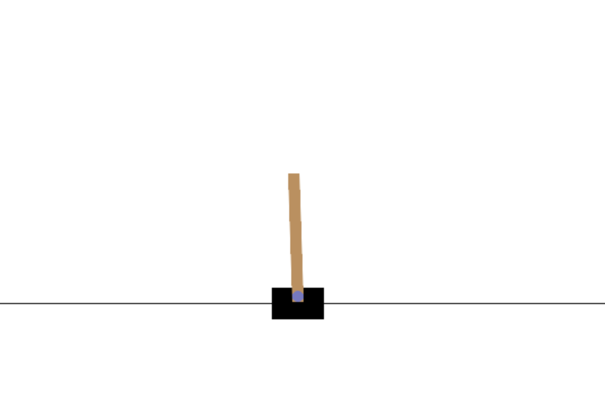
The gymnasium package for Python provides several environments (APIs) that are suited for RL agents to be trained. CartPole is a relatively simple game that requires an agent to balance a pole on a cart by pushing the cart to the left or right. This section illustrates the API for the game, that is the environment, and shows how to implement a DQL agent in Python that can learn to play the game perfectly.

2.4.1. The Game Environment

The gymnasium package is installed as follows:

pip install gymnasium

Details about the CartPole game are found at https://gymnasium.farama.org. The first step is the creation of an environment object:

In [1]: import gymnasium as gym

In [2]: env = gym.make('CartPole-v1')

This object allows the interaction via simple method calls. For example, it allows us to see how many actions are feasible (action space), to sample random actions, or to get more information about the state description (observation space):

In [3]: env.action_space
Out[3]: Discrete(2)

In [4]: env.action_space.n  (1)
Out[4]: 2

In [5]: [env.action_space.sample() for _ in range(10)]  (1)
Out[5]: [1, 0, 1, 0, 0, 0, 0, 0, 0, 0]

In [6]: env.observation_space
Out[6]: Box([-4.8000002e+00 -3.4028235e+38 -4.1887903e-01 -3.4028235e+38],
         [4.8000002e+00 3.4028235e+38 4.1887903e-01 3.4028235e+38], (4,),
         float32)

In [7]: env.observation_space.shape  (2)
Out[7]: (4,)

1	Two actions, `0` and `1`, are possible.
2	The state is described by four parameters.

The environment allows an agent to take one of two actions:

0: Push the cart to the left.
1: Push the cart to the right.

The environment models the state of the game through four physical parameters:

Cart position
Cart velocity
Pole angle
Pole angular velocity

CartPole game shows a visual representation of a state of the CartPole game.

Figure 1. CartPole game

To play the game, the environment is first reset, leading by default to a randomized initial state. Every action steps the environment forward to the next state:

In [8]: env.reset(seed=100)  (1)
        # cart position, cart velocity, pole angle, pole angular velocity
Out[8]: (array([ 0.03349816,  0.0096554 , -0.02111368, -0.04570484],
         dtype=float32),
         {})

In [9]: env.step(0)  (2)
Out[9]: (array([ 0.03369127, -0.18515752, -0.02202777,  0.24024247],
         dtype=float32),
         1.0,
         False,
         False,
         {})

In [10]: env.step(1)  (2)
Out[10]: (array([ 0.02998812,  0.01027205, -0.01722292, -0.05930644],
          dtype=float32),
          1.0,
          False,
          False,
          {})

1	Resets the environment, using a `seed` value for the random number generator.
2	Steps the environment one step forward by taking one of two actions.

The returned tuple contains the following data:

New state
Reward
Terminated
Truncated
Additional data

The game can be played until True is returned for “terminated”. For every step, the agent receives a reward of 1. The more steps, the higher the total reward. The objective of an RL agent is to maximize the total reward or to achieve a minimum reward, for example.

2.4.2. A Random Agent

It is straightforward to implement an agent that only takes random actions. It cannot be expected that the agent will achieve a high total reward on average. However, every once in a while such an agent might be lucky.

The following Python code implements a random agent and collects the results from a larger number of games played:

In [11]: class RandomAgent:
             def __init__(self):
                 self.env = gym.make('CartPole-v1')
             def play(self, episodes=1):
                 self.trewards = list()
                 for e in range(episodes):
                     self.env.reset()
                     for step in range(1, 100):
                         a = self.env.action_space.sample()
                         state, reward, done, trunc, info = self.env.step(a)
                         if done:
                             self.trewards.append(step)
                             break

In [12]: ra = RandomAgent()

In [13]: ra.play(15)

In [14]: ra.trewards
Out[14]: [18, 28, 17, 25, 16, 41, 21, 19, 22, 9, 11, 13, 15, 14, 11]

In [15]: round(sum(ra.trewards) / len(ra.trewards), 2)  (1)
Out[15]: 18.67

1	Average reward for the random agent.

The results illustrate that the random agent does not survive that long. The total reward might be somewhat above 20 or below. In rare cases, a relatively high total reward — for example, close to 50 — might be observed (called a lucky punch).

2.4.3. The DQL Agent

This sub-section implements a DQL agent in multiple steps. This allows for a more detailed discussion of the single elements that make up the agent. Such an approach seems justified because this DQL agent will serve as a blueprint for the DQL agent that will be applied to financial problems.

To get started, the following Python code first does all the required imports and customizes TensorFlow.

In [16]: import os
         import random
         import warnings
         import numpy as np
         import tensorflow as tf
         from tensorflow import keras
         from collections import deque
         from keras.layers import Dense
         from keras.models import Sequential

In [17]: warnings.simplefilter('ignore')
         os.environ['TF_CPP_MIN_LOG_LEVEL'] = '3'
         os.environ['PYTHONHASHSEED'] = '0'

In [18]: from tensorflow.python.framework.ops import disable_eager_execution
         disable_eager_execution()  (1)

In [19]: opt = keras.optimizers.legacy.Adam(learning_rate=0.0001)  (2)

In [20]: random.seed(100)
         tf.random.set_seed(100)

1	Speeds up the training of the neural network.
2	Defines the optimizer to be used for the training.

The following Python code shows the initial part of the DQLAgent class. Among other things, it defines the major parameters and instantiates the DNN that is used for representing the optimal action policy.

In [21]: class DQLAgent:
             def __init__(self):
                 self.epsilon = 1.0  (1)
                 self.epsilon_decay = 0.9975  (2)
                 self.epsilon_min = 0.1  (3)
                 self.memory = deque(maxlen=2000)  (4)
                 self.batch_size = 32  (5)
                 self.gamma = 0.9  (6)
                 self.trewards = list()  (7)
                 self.max_treward = 0  (8)
                 self._create_model()  (9)
                 self.env = gym.make('CartPole-v1')  (10)
             def _create_model(self):
                 self.model = Sequential()
                 self.model.add(Dense(24, activation='relu', input_dim=4))
                 self.model.add(Dense(24, activation='relu'))
                 self.model.add(Dense(2, activation='linear'))
                 self.model.compile(loss='mse', optimizer=opt)

1	The initial ratio `epsilon` with which exploration is implemented.
2	The factor by which `epsilon` is diminished.
3	The minimum value for `epsilon`.
4	The `deque` object which collects past experiences.^[13]
5	The number of experiences used for replay.
6	The factor to discount future rewards.
7	A `list` object to collect total rewards.
8	A parameter to store the maximum total reward achieved.
9	Initiates the instantiation of the DNN.
10	Instantiates the `CartPole` environment.

The next part of the DQLAgent class implements the .act() and .replay() methods for choosing an action and updating the DNN (optimal action policy) given past experiences.

In [22]: class DQLAgent(DQLAgent):
             def act(self, state):
                 if random.random() < self.epsilon:
                     return self.env.action_space.sample()  (1)
                 return np.argmax(self.model.predict(state)[0])  (2)
             def replay(self):
                 batch = random.sample(self.memory, self.batch_size)  (3)
                 for state, action, next_state, reward, done in batch:
                     if not done:
                         reward += self.gamma * np.amax(
                             self.model.predict(next_state)[0])  (4)
                     target = self.model.predict(state)  (5)
                     target[0, action] = reward  (6)
                     self.model.fit(state, target, epochs=2, verbose=False)  (7)
                 if self.epsilon > self.epsilon_min:
                     self.epsilon *= self.epsilon_decay  (8)

1	Chooses a random action.
2	Chooses an action according to the (current) optimal policy.
3	Randomly chooses a batch of past experiences for replay.
4	Combines the immediate and discounted future reward.
5	Generates the values for the state-action pairs.
6	Updates the value for the relevant state-action pair.
7	Trains/updates the DNN to account for the updated value.
8	Reduces `epsilon` by the `epsilon_decay` factor.

The major elements are available to implement the core part of the DQLAgent class: the .learn() method which controls the interaction of the agent with the environment and the updating of the optimal policy. It also generates printed output to monitor the learning of the agent.

In [23]: class DQLAgent(DQLAgent):
             def learn(self, episodes):
                 for e in range(1, episodes + 1):
                     state, _ = self.env.reset()  (1)
                     state = np.reshape(state, [1, 4])  (2)
                     for f in range(1, 5000):
                         action = self.act(state)  (3)
                         next_state, reward, done, trunc, _ = self.env.step(action)  (4)
                         next_state = np.reshape(next_state, [1, 4])  (2)
                         self.memory.append(
                             [state, action, next_state, reward, done])  (4)
                         state = next_state  (5)
                         if done or trunc:
                             self.trewards.append(f)  (6)
                             self.max_treward = max(self.max_treward, f)  (7)
                             templ = f'episode={e:4d} | treward={f:4d}'
                             templ += f' | max={self.max_treward:4d}'
                             print(templ, end='\r')
                             break
                     if len(self.memory) > self.batch_size:
                         self.replay()  (8)
                 print()

1	The environment is reset.
2	The state object is reshaped.^[14]
3	An action is chosen according to the `.act()` method, given the current state.
4	The relevant data points are collected for replay.
5	The `state` variable is updated to the current state.
6	Once terminated, the total reward is collected.
7	The maximum total reward is updated if necessary.
8	Replay is initiated as long as there are enough past experiences.

With the following Python code, the class is complete. It implements the .test() method that allows the testing of the agent without exploration.

In [24]: class DQLAgent(DQLAgent):
             def test(self, episodes):
                 for e in range(1, episodes + 1):
                     state, _ = self.env.reset()
                     state = np.reshape(state, [1, 4])
                     for f in range(1, 5001):
                         action = np.argmax(self.model.predict(state)[0])  (1)
                         state, reward, done, trunc, _ = self.env.step(action)
                         state = np.reshape(state, [1, 4])
                         if done or trunc:
                             print(f, end=' ')
                             break

1	For testing, only actions according to the optimal policy are chosen.

The DQL agent in the form of the completed DQLAgent Python class can interact with the CartPole environment to improve its capabilities in playing the game — as measured by the rewards achieved.

In [25]: agent = DQLAgent()

In [26]: %time agent.learn(1500)
         episode=1500 | treward= 224 | max= 500
         CPU times: user 1min 52s, sys: 21.7 s, total: 2min 14s
         Wall time: 1min 46s

In [27]: agent.epsilon
Out[27]: 0.09997053357470892

In [28]: agent.test(15)
         500 373 326 500 348 303 500 330 392 304 250 389 249 204 500

At first glance, it is clear that the DQL agent consistently outperforms the random agent by a large margin. Therefore, luck can’t be at work. On the other hand, without additional context, it is not clear whether the agent is a mediocre, good, or very good one.

In the documentation for the CartPole environment, you find that the threshold for total rewards is 475. This means that everything above 475 is considered to be good. By default, the environment is truncated at 500 meaning that reaching that level is considered to be a “success” for the game. However, the game can be played beyond 500 steps/rewards which might make the training of the DQL agent more efficient.

2.5. Q-Learning vs. Supervised Learning

At the core of DQL is a DNN that resembles those often used and seen in supervised learning. Against this background, what are the major differences between these two approaches in machine learning?

To get started, the objective of both approaches is different. Concerning DQL, the objective is to learn an optimal action policy that maximizes total reward (or minimizes total penalties, for example). On the other hand, supervised learning aims at learning a mapping between features and labels.

Secondly, in DQL the data is generated through interaction and in a sequential fashion. The sequence of the data in general matters, like the sequence of moves in chess matter. In supervised learning, the data set is generally given upfront in the form of (expert-)labeled data sets and the sequence often does not matter at all. Supervised learning, in that sense, is based on a given set of correct examples while DQL needs to generate appropriate data sets through interaction step-by-step.

Thirdly, in DQL feedback generally comes delayed given an action taken now. A DQL agent playing a game might not know until many steps later whether a current action is reward maximizing or not. The algorithm, however, makes sure that delayed feedback backpropagates in time through replay and updating of the DNN. In supervised learning, all relevant examples exist upfront and immediate feedback is available as to whether the algorithm gets the mapping between features and labels correct or not.

In summary, while DNNs might be at the core of both DQL and supervised learning they differ in fundamental ways in terms of their objective, the data they use, and the feedback their learning is based on.

2.6. Conclusions

Decision problems in economics and finance are manifold. One of the most important types is dynamic programming. This chapter classifies decision problems along the lines of different binary characteristics (such as discrete or continuous action space) and introduces dynamic programming as an important algorithm to solve dynamic decision problems in discrete time.

Deep Q-learning is formalized and illustrated based on a simple game — CartPole from the gymnasium Python environment. The major goals in this regard are to illustrate the API-based interaction with an environment suited for RL and the implementation of a DQL agent in the form of a self-contained Python class.

The next chapter develops a simple financial environment that mimics the behavior of the CartPole environment so that the DQL agent from this chapter can learn to play a financial prediction game.

2.7. References

Articles and books cited in this chapter:

Duffie, Darrell (1988): Security Markets: Stochastic Models. Academic Press, Boston.
Duffie, Darrell (2001): Dynamic Asset Pricing Theory. 3rd ed., Princeton University Press, Princeton.
Li, Yuxi (2018): “Deep Reinforcement Learning: An Overview.” https://doi.org/10.48550/arXiv.1701.07274.
Sargent, Thomas and John Stucharski (2023): Dynamic Programming. https://dp.quantecon.org/.
Stucharski, John (2009): Economic Dynamics—Theory and Computation. MIT Press, Cambridge and London.
Sundaram, Rangarajan (1996): A First Course in Optimization Theory. Cambridge University Press, Cambridge.
Watkins, Christopher (1989): Learning from Delayed Rewards. Ph.D. thesis, University of Cambridge.
Watkins, Christopher and Peter Dayan (1992): “Q-Learning.” Machine Learning, Vol. 8, 279-282.

3. Financial Q-Learning

Today’s algorithmic trading programs are relatively simple and make only limited use of AI. This is sure to change.

— Murray Shanahan (2015)

The previous chapter shows that a DQL agent can learn to play the game of CartPole quite well. What about financial applications? As this chapter shows, the agent can also learn to play a financial game that is about predicting the future movement in a financial market. To this end, this chapter implements a finance environment that mimics the behavior of the CartPole environment and trains the DQL agent from the previous chapter based on this finance environment.

This chapter is quite brief, but it illustrates an important point: with the appropriate environment, DQL can be applied to financial problems basically in the same way as it is applied to games and in other domains. Finance Environment develops step-by-step the Finance class that mimics the behavior of the CartPole class. DQL Agent slightly adjusts the DQLAgent class from CartPole as an Example. The adjustments are made to reflect the new context. The DQL agent can learn to predict future market movements with a significant margin over the baseline accuracy of 50%. Where the Analogy Fails finally discusses the major issues of the modeling approach and the Finance class when compared, for example, to a gaming environment such as the CartPole game.

3.1. Finance Environment

The idea for the finance environment to be implemented in the following is that of a prediction game. The environment uses static historical financial time series data to generate the states of the environment and the value to be predicted by the DQL agent. The state is given by four floating point numbers representing the four most recent data points in the time series — such as normalized price or return values. The value to be predicted is either 0 or 1. Here, 0 means that the financial time series value drops to a lower level (“market goes down”) and 1 means that the time series value rises to a higher level (“market goes up”).

To get started, the following Python class implements the behavior of the env.action_space object for the generation of random actions. The DQL agent relies on this capability in the context of exploration:

In [1]: import os
        import random

In [2]: random.seed(100)
        os.environ['PYTHONHASHSEED'] = '0'

In [3]: class ActionSpace:
            def sample(self):
                return random.randint(0, 1)

In [4]: action_space = ActionSpace()

In [5]: [action_space.sample() for _ in range(10)]
Out[5]: [0, 1, 1, 0, 1, 1, 1, 0, 0, 0]

The Finance class, which is at the core of this chapter, implements the idea of the prediction game as described before. It starts with the definition of important parameters and objects:

In [6]: import numpy as np
        import pandas as pd

In [7]: class Finance:
            url = 'https://certificate.tpq.io/rl4finance.csv'  (1)
            def __init__(self, symbol, feature, min_accuracy=0.485, n_features=4):
                self.symbol = symbol  (2)
                self.feature = feature  (3)
                self.n_features = n_features  (4)
                self.action_space = ActionSpace()  (5)
                self.min_accuracy = min_accuracy  (6)
                self._get_data()  (7)
                self._prepare_data()  (8)
            def _get_data(self):
                self.raw = pd.read_csv(self.url,
                        index_col=0, parse_dates=True)  (7)

1	The URL for the data set to be used (can be replaced).
2	The symbol for the time series to be used for the prediction game.
3	The type of feature to be used to define the state of the environment.
4	The number of feature values to be provided to the agent.
5	The `ActionSpace` object that is used for random action sampling.
6	The minimum prediction accuracy required for the agent to continue with the prediction game.
7	The retrieval of the financial time series data from the remote source.
8	The method call for the data preparation.

The data set used in this class allows the selection of the following financial instruments:

AAPL.O | Apple Stock
MSFT.O | Microsoft Stock
INTC.O | Intel Stock
AMZN.O | Amazon Stock
GS.N   | Goldman Sachs Stock
SPY    | SPDR S&P 500 ETF Trust
.SPX   | S&P 500 Index
.VIX   | VIX Volatility Index
EUR=   | EUR/USD Exchange Rate
XAU=   | Gold Price
GDX    | VanEck Vectors Gold Miners ETF
GLD    | SPDR Gold Trust

A key method of the Finance class is the one for preparing the data for both the state description (features) and the prediction itself (labels). The state data is provided in normalized form, which is known to improve the performance of DNNs. From the implementation, it is obvious that the financial time series data is used in a static, non-random way. When the environment is reset to the initial state, it is always the same initial state.

In [8]: class Finance(Finance):
            def _prepare_data(self):
                self.data = pd.DataFrame(self.raw[self.symbol]).dropna()  (1)
                self.data['r'] = np.log(self.data / self.data.shift(1))  (2)
                self.data['d'] = np.where(self.data['r'] > 0, 1, 0)  (3)
                self.data.dropna(inplace=True)  (4)
                self.data_ = (self.data - self.data.mean()) / self.data.std()  (5)
            def reset(self):
                self.bar = self.n_features  (6)
                self.treward = 0  (7)
                state = self.data_[self.feature].iloc[
                    self.bar - self.n_features:self.bar].values  (8)
                return state, {}

1	Selects the relevant time series data from the `DataFrame` object.
2	Generates a log return time series from the price time series.
3	Generates the binary, directional data to be predicted from the log returns.
4	Gets rid of all those rows in the `DataFrame` object that contain `NaN` (“not a number”) values.
5	Applies Gaussian normalization to the data.
6	Sets the current bar (position in the time series) to the value for the number of feature values.
7	Resets the total reward value to zero.
8	Generates the initial state object to be returned by the method.

The following Python code finally implements the .step() method which moves the environment from one state to the next or signals that the game is terminated. One key idea is to check for the current prediction accuracy of the agent and to compare it to a minimum required accuracy. The purpose is to avoid that the agent simply plays along even if its current performance is much worse than, say, that of a random agent.

In [9]: class Finance(Finance):
            def step(self, action):
                if action == self.data['d'].iloc[self.bar]:  (1)
                    correct = True
                else:
                    correct = False
                reward = 1 if correct else 0  (2)
                self.treward += reward  (3)
                self.bar += 1  (4)
                self.accuracy = self.treward / (self.bar - self.n_features)  (5)
                if self.bar >= len(self.data):  (6)
                    done = True
                elif reward == 1:  (7)
                    done = False
                elif (self.accuracy < self.min_accuracy) and (self.bar > 15):  (8)
                    done = True
                else:
                    done = False
                next_state = self.data_[self.feature].iloc[
                    self.bar - self.n_features:self.bar].values  (9)
                return next_state, reward, done, False, {}

1	Checks whether the prediction (“action”) is correct.
2	Assigns a reward of `+1` or `0` depending on correctness.
3	Increases the total reward accordingly.
4	The bar value is increased to move the environment forward on the time series.
5	The current accuracy is calculated.
6	Checks whether the end of the data set is reached.
7	Checks whether the prediction was correct.
8	Checks whether the current accuracy is above the minimum required accuracy.
9	Generates the next state object to be returned by the method.

This completes the Finance class and allows the instantiation of objects based on the class as in the following Python code. The code also lists the available symbols in the financial data set used. It further illustrates that either normalized price or log returns data can be used to describe the state of the environment.

In [10]: fin = Finance(symbol='EUR=', feature='EUR=')  (1)

In [11]: list(fin.raw.columns)  (2)
Out[11]: ['AAPL.O',
          'MSFT.O',
          'INTC.O',
          'AMZN.O',
          'GS.N',
          '.SPX',
          '.VIX',
          'SPY',
          'EUR=',
          'XAU=',
          'GDX',
          'GLD']

In [12]: fin.reset()
         # four lagged, normalized price points
Out[12]: (array([2.74844931, 2.64643904, 2.69560062, 2.68085214]), {})

In [13]: fin.action_space.sample()
Out[13]: 1

In [14]: fin.step(fin.action_space.sample())
Out[14]: (array([2.64643904, 2.69560062, 2.68085214, 2.63046153]), 0, False,
          False, {})

In [15]: fin = Finance('EUR=', 'r')  (3)

In [16]: fin.reset()
         # four lagged, normalized log returns
Out[16]: (array([-1.19130476, -1.21344494,  0.61099805, -0.16094865]), {})

1	Specifies the feature type to be normalized prices.
2	Shows the available symbols in the data set used.
3	Specifies the feature type to be normalized returns.

To illustrate the interaction with the Finance environment, a random agent can again be considered. The total rewards that the agent achieves are, of course, quite low. They are slightly above 20 on average. This needs to be compared with the length of the data set which has more than 2,500 data points. In other words, a total reward of 2,500 or more is possible.

In [17]: class RandomAgent:
             def __init__(self):
                 self.env = Finance('EUR=', 'r')
             def play(self, episodes=1):
                 self.trewards = list()
                 for e in range(episodes):
                     self.env.reset()
                     for step in range(1, 100):
                         a = self.env.action_space.sample()
                         state, reward, done, trunc, info = self.env.step(a)
                         if done:
                             self.trewards.append(step)
                             break

In [18]: ra = RandomAgent()

In [19]: ra.play(15)

In [20]: ra.trewards
Out[20]: [17, 13, 17, 12, 12, 12, 13, 23, 31, 13, 12, 15]

In [21]: round(sum(ra.trewards) / len(ra.trewards), 2)  (1)
Out[21]: 15.83

In [22]: len(fin.data)  (2)
Out[22]: 2607

1	Average reward for the random agent.
2	Length of the data set which equals roughly the maximum total reward.

3.2. DQL Agent

Equipped with the Finance environment, it is straightforward to let the DQL agent (DQLAgent class from The DQL Agent) play the financial prediction game.

The following Python code takes care of the required imports and configurations.

In [23]: import os
         import random
         import warnings
         import numpy as np
         import tensorflow as tf
         from tensorflow import keras
         from collections import deque
         from keras.layers import Dense
         from keras.models import Sequential

In [24]: warnings.simplefilter('ignore')
         os.environ['TF_CPP_MIN_LOG_LEVEL'] = '3'

In [25]: from tensorflow.python.framework.ops import disable_eager_execution
         disable_eager_execution()

In [26]: opt = keras.optimizers.legacy.Adam(learning_rate=0.0001)

For the sake of completeness, the following code shows the DQLAgent class as a whole. It is basically the same code as in The DQL Agent with some minor adjustments for the context of this chapter.

In [27]: class DQLAgent:
             def __init__(self, symbol, feature, min_accuracy, n_features=4):
                 self.epsilon = 1.0
                 self.epsilon_decay = 0.9975
                 self.epsilon_min = 0.1
                 self.memory = deque(maxlen=2000)
                 self.batch_size = 32
                 self.gamma = 0.5
                 self.trewards = list()
                 self.max_treward = 0
                 self.n_features = n_features
                 self._create_model()
                 self.env = Finance(symbol, feature,
                             min_accuracy, n_features)  (1)
             def _create_model(self):
                 self.model = Sequential()
                 self.model.add(Dense(24, activation='relu',
                                      input_dim=self.n_features))
                 self.model.add(Dense(24, activation='relu'))
                 self.model.add(Dense(2, activation='linear'))
                 self.model.compile(loss='mse', optimizer=opt)
             def act(self, state):
                 if random.random() < self.epsilon:
                     return self.env.action_space.sample()
                 return np.argmax(self.model.predict(state)[0])
             def replay(self):
                 batch = random.sample(self.memory, self.batch_size)
                 for state, action, next_state, reward, done in batch:
                     if not done:
                         reward += self.gamma * np.amax(
                             self.model.predict(next_state)[0])
                     target = self.model.predict(state)
                     target[0, action] = reward
                     self.model.fit(state, target, epochs=1, verbose=False)
                 if self.epsilon > self.epsilon_min:
                     self.epsilon *= self.epsilon_decay
             def learn(self, episodes):
                 for e in range(1, episodes + 1):
                     state, _ = self.env.reset()
                     state = np.reshape(state, [1, self.n_features])
                     for f in range(1, 5000):
                         action = self.act(state)
                         next_state, reward, done, trunc, _ = self.env.step(action)
                         next_state = np.reshape(next_state, [1, self.n_features])
                         self.memory.append(
                             [state, action, next_state, reward, done])
                         state = next_state
                         if done:
                             self.trewards.append(f)
                             self.max_treward = max(self.max_treward, f)
                             templ = f'episode={e:4d} | treward={f:4d}'
                             templ += f' | max={self.max_treward:4d}'
                             print(templ, end='\r')
                             break
                     if len(self.memory) > self.batch_size:
                         self.replay()
                 print()
             def test(self, episodes):
                 ma = self.env.min_accuracy  (2)
                 self.env.min_accuracy = 0.5  (3)
                 for e in range(1, episodes + 1):
                     state, _ = self.env.reset()
                     state = np.reshape(state, [1, self.n_features])
                     for f in range(1, 5001):
                         action = np.argmax(self.model.predict(state)[0])
                         state, reward, done, trunc, _ = self.env.step(action)
                         state = np.reshape(state, [1, self.n_features])
                         if done:
                             print(f'total reward={f} | accuracy={self.env.accuracy:.3f}')
                             break
                 self.env.min_accuracy = ma  (2)

1	Defines the `Finance` environment object as a class attribute.
2	Captures and resents the original minimum accuracy for the `Finance` environment.
3	Redefines the minimum accuracy for testing purposes.

As the following Python code shows, the DQLAgent learns to predict the next market movement with an accuracy of significantly above 50%.

In [28]: random.seed(250)
         tf.random.set_seed(250)

In [29]: agent = DQLAgent('EUR=', 'r', 0.495, 4)

In [30]: %time agent.learn(250)
         episode= 250 | treward=  12 | max=2603
         CPU times: user 18.6 s, sys: 3.15 s, total: 21.8 s
         Wall time: 18.2 s

In [31]: agent.test(5)  (1)
         total reward=2603 | accuracy=0.525
         total reward=2603 | accuracy=0.525
         total reward=2603 | accuracy=0.525
         total reward=2603 | accuracy=0.525
         total reward=2603 | accuracy=0.525

1	Test results are all the same given the static data set.

3.3. Where the Analogy Fails

The Finance environment as introduced in Finance Environment has one major goal: to exactly replicate the API of the CartPole environment. This goal is relatively easily achieved, allowing the DQL agent from the previous chapter to learn the financial prediction game. This is an accomplishment and insight in and of itself: a DQL agent can learn to play different games — even a large number of them.

However, the Finance environment brings two major, intertwined drawbacks with it: limited data and no impact of actions. This section discusses them in some detail.

3.3.1. Limited Data

The first drawback is that the environment is based on a static, deterministic data set. Whenever the environment is reset it starts at the same initial state and moves step-by-step through the same states afterward, independent of the action (prediction) of the DQL agent.

This is in stark contrast to the CartPole environment, which by default generates a random initial state. Given the random initial state, the whole set of ensuing states afterward can be considered to be a sequence of random states since they always differ given a new random initial state.

Here, it is important to note that the transition from one state to another is deterministic. However, all sequences of states will differ due to the initial state being random. In a certain sense, the sequence of states as a whole inherits its randomness from the initial state.

Working with static data sets limits the training data in a severe fashion. Although the data set has more than 2,500 data points it is just one data set. The situation is as if an RL agent should learn to play chess based on a single historical game only, which it can go through over and over again. It is also comparable to a student who wants to prepare for an upcoming mathematics exam but only has one mathematics problem available to study and prepare with. Too little data is not only a problem in RL but obviously in machine learning and deep learning in general.

Another thought should be outlined here as well. Even if one adds other historical financial time series to the training data set or if one uses, say, historical intraday data instead of end-of-day data, the problem of “limited financial data” persists. It might not be as severe as in the context of the Finance environment, but the problem would still play an important role.

Too Little Data

The success or failure of a DQL agent often depends on the availability of large amounts of or even infinite data. When playing board games such as chess, for example, the available data (experiences made) is practically infinite because an agent can play a very large number of games against itself. Financial data in and of itself is limited by definition.

3.3.2. No Impact

In RL with DQL agents, it is often assumed or expected that the next state of an environment depends on the action chosen by the agent at least to some extent. In chess, it is clear that the next board position depends on the move of the player or the DQL agent trying to learn the game. In CartPole, the agent influences all four parameters of the next state — cart position, cart velocity, pole angle, angular velocity — by pushing the cart to the left or right.

In The Book of Why, the authors explain that there are three layers based on which causal relationships can be learned and formulated. The first is data that can be observed, processed, and analyzed. For example, this might lead to insights concerning the correlation between two related quantities. But as is often pointed out, correlation is not necessarily causation.

To get deeper insights into what might really cause a phenomenon or an observation, one needs the other two layers in general. The second layer is about interventions. In the real world, you can in general expect that an action has some impact. Whether I exercise regularly or not, it should make a difference in the evolution of my weight and health, for example. This is comparable to the CartPole environment for which every action has a direct impact.

For the Finance environment, the next state is completely independent of the prediction (action) of the DQL agent. In this context, it might be acceptable that way, because, after all, what impact shall a prediction of a DQL agent (or a human analyst to this end) have on the evolution of the EUR/USD exchange rate or the Apple share price? In finance, it is routinely assumed, that agents are “infinitesimally small” and therefore cannot impact financial markets through trading or other financial decisions.

In reality, of course, large financial institutions often have a significant influence on financial markets, for example, when executing a large order or block trade. In such a context, feedback effects of actions would be highly relevant for the learning of optimal execution strategies, for instance.

Going one level higher and recalling what RL is about at its core, it should also be clear that the consequences of actions should play an important role. How should “reinforcement” otherwise be happening if the consequences of actions have no effect? The situation is comparable to a student receiving the same feedback from his parents no matter whether they have an A or D grade in a mathematics exam. For a comprehensive discussion about the role consequences of actions play for human beings and animals alike, see the book The Science of Consequences by Schneider (2012).

The third layer is about counterfactuals. This implies that an agent possesses the capabilities to imagine hypothetical states for an environment and to hypothetically simulate the impact that a hypothetical action might have. This probably cannot be expected entirely from a DQL agent as discussed in this book. It might be something for which an artificial general intelligence (AGI) might be required.^[15] On a more simple level, one could interpret the simulation of a hypothetical future action that is optimal as coming up with a counterfactual. The DQL agent does not, however, hypothesize about possible states that it has not experienced before.

No Impact

In this book, it is usually assumed that a DQL agent’s actions have no direct effect on the next state. A state is given, and, independent of which action the agent chooses, the next state is revealed to the agent. This holds for static historical data sets or those generated in Data Augmentation based on adding noise, leveraging simulation techniques, or generative adversarial networks.

3.4. Conclusions

This chapter develops a simple financial environment that allows the DQL agent from the previous chapter (with some minor adjustments) to learn a financial prediction game. The environment is based on real historical financial price data. The DQL agent learns to predict the future movement of the market (the price of the financial instrument chosen) with an accuracy that is significantly above the 50% baseline level.

While the financial environment developed in this chapter mimics the major elements of the API as provided by the CartPole environment it lacks two important elements: the training data set is limited to a single, static time series only and the actions of the DQL agents do not impact the state of the environment.

Data Augmentation focuses on the major problem of limited financial data and introduces data augmentation approaches that allow to generate a basically unlimited number of financial time series.

3.5. References

Books cited in this chapter:

Hilpisch, Yves (2020): Artificial Intelligence for Finance: A Python-based Guide. O’Reilly Media.
Pearl, Judea and Dana Mackkenzie (2018): The Book of Why: The New Science of Cause and Effect. Penguin Science.
Shanahan, Murray (2015): The Technological Singularity. MIT Press, Cambridge & London.
Schneider, Susan (2012). The Science of Consequences: How They Affect Genes, Change the Brain, and Impact Our World. Prometheus Books, Amherst.

Data Augmentation

The second part of the book covers concepts and approaches to generate data for financial deep Q-learning:

Simulated Data implements data generation approaches based on Monte Carlo simulation. One approach is to add white noise to an existing financial time series. Another one is to simulate financial time series data based on a financial model (stochastic differential equation).
Generated Data shows how to use generative adversarial networks (GANs) from artificial intelligence (AI), or more specifically from deep learning (DL), to generate financial time series data that is consistent with and statistically indistinguishable from the target financial time series. Such a target time series can be the historical price series for the share of a company stock (think Apple shares) or the historical foreign exchange quotes (think EUR/USD exchange rate).

4. Simulated Data

It is often said that data is the new oil, but this analogy is not quite right. Oil is a finite resource that must be extracted and refined, whereas data is an infinite resource that is constantly being generated and refined.

— Halevy et al. (2009)

A major drawback of the financial environment as introduced in the previous chapter is that it relies by default on a single, historical financial time series. This is a too-limited data set to train a deep Q-learning (DQL) agent. It is like training an AI on a single game of chess and expecting it to perform well overall in chess.

This chapter introduces simulation-based approaches to augment the available data for the training of a DQL agent. The first approach, as introduced in Noisy Time Series Data, is to add random noise to a static financial time series. Although it is commonly agreed upon that financial times data generally already contains noise — as compared to price movements or returns that are information-induced — the idea is to train the agent on a large number of “similar” time series in the hope that it learns to distinguish information from noise.

The second approach, discussed in Simulated Time Series Data, is to generate financial time series data through simulation under certain constraints and assumptions. In general, a stochastic differential equation is assumed for the dynamics of the time series. The time series is then simulated given a discretization scheme and appropriate boundary conditions. This is one of the core numerical approaches used in computational finance to price financial derivatives or to manage financial risks, for example (see Glasserman (2004)).

Both data augmentation methods discussed in this chapter make it possible to generate an unlimited amount of training, validation, and test data for reinforcement learning.

4.1. Noisy Time Series Data

This section adjusts the first Finance environment from Finance Environment to add white noise, which is normally distributed data, to the original financial time series. First, the helper class for the action space:

In [1]: class ActionSpace:
            def sample(self):
                return random.randint(0, 1)

The new NoisyData environment class only requires a few adjustments compared to the original Finance class. In the following Python code, two parameters are added to the initialization method:

In [2]: import numpy as np
        import pandas as pd
        from numpy.random import default_rng  (1)

In [3]: rng = default_rng(seed=100)  (1)

In [4]: class NoisyData:
            url = 'https://certificate.tpq.io/findata.csv'
            def __init__(self, symbol, feature, n_features=4,
                         min_accuracy=0.485, noise=True,
                         noise_std=0.001):
                self.symbol = symbol
                self.feature = feature
                self.n_features = n_features
                self.noise = noise  (2)
                self.noise_std = noise_std  (3)
                self.action_space = ActionSpace()
                self.min_accuracy = min_accuracy
                self._get_data()
                self._prepare_data()
            def _get_data(self):
                self.raw = pd.read_csv(self.url,
                        index_col=0, parse_dates=True)

1	The random number generator is imported and initialized.
2	The flag that specifies whether noise is added or not.
3	The noise level to be used when adjusting the data; it is to be given in % of the price level.

The following part of the Python class code is the most important one. It is where the noise is added to the original time series data:

In [5]: class NoisyData(NoisyData):
            def _prepare_data(self):
                self.data = pd.DataFrame(self.raw[self.symbol]).dropna()
                if self.noise:
                    std = self.data.mean() * self.noise_std  (1)
                    self.data[self.symbol] = (self.data[self.symbol] +
                        rng.normal(0, std, len(self.data)))  (2)
                self.data['r'] = np.log(self.data / self.data.shift(1))
                self.data['d'] = np.where(self.data['r'] > 0, 1, 0)
                self.data.dropna(inplace=True)
                ma, mi = self.data.max(), self.data.min()  (3)
                self.data_ = (self.data - mi) / (ma - mi)  (3)
            def reset(self):
                if self.noise:
                    self._prepare_data()  (4)
                self.bar = self.n_features
                self.treward = 0
                state = self.data_[self.feature].iloc[
                    self.bar - self.n_features:self.bar].values
                return state, {}

1	The standard deviation for the noise is calculated in absolute terms.
2	The white noise is added to the time series data.
3	The features data is normalized through min-max scaling.
4	A new noisy time series data set is generated.

Information vs. Noise

Generally, it is assumed that financial time series data includes a certain amount of noise already. Investopedia defines noise as follows: “Noise refers to information or activity that confuses or misrepresents genuine underlying trends.” In this section, we take the historical price series as given and actively add noise to it. The idea is that a DQL agent learns about the fundamental price and/or return trends embodied by the historical data set.

The final part of the Python class, the .step() method, can remain unchanged:

In [6]: class NoisyData(NoisyData):
            def step(self, action):
                if action == self.data['d'].iloc[self.bar]:
                    correct = True
                else:
                    correct = False
                reward = 1 if correct else 0
                self.treward += reward
                self.bar += 1
                self.accuracy = self.treward / (self.bar - self.n_features)
                if self.bar >= len(self.data):
                    done = True
                elif reward == 1:
                    done = False
                elif (self.accuracy < self.min_accuracy and
                      self.bar > self.n_features + 15):
                    done = True
                else:
                    done = False
                next_state = self.data_[self.feature].iloc[
                    self.bar - self.n_features:self.bar].values
                return next_state, reward, done, False, {}

Every time the financial environment is reset, a new time series is created by adding noise to the original time series. The following Python code illustrates this numerically:

In [7]: fin = NoisyData(symbol='EUR=', feature='EUR=',
                        noise=True, noise_std=0.005)

In [8]: fin.reset()  (1)
Out[8]: (array([0.79295659, 0.81097879, 0.78840972, 0.80597193]), {})

In [9]: fin.reset()  (1)
Out[9]: (array([0.80642276, 0.77840938, 0.80096369, 0.76938581]), {})

In [10]: fin = NoisyData('EUR=', 'r', n_features=4,
                         noise=True, noise_std=0.005)

In [11]: fin.reset()  (2)
Out[11]: (array([0.54198375, 0.30674865, 0.45688528, 0.52884033]), {})

In [12]: fin.reset()  (2)
Out[12]: (array([0.37967631, 0.40190291, 0.49196183, 0.47536065]), {})

1	Different initial states for the normalized price data.
2	Different initial states for the normalized returns data.

Finally, the following code visualizes several noisy time series data sets (see Noisy time series data for half a year):

In [13]: from pylab import plt, mpl
         plt.style.use('seaborn-v0_8')
         mpl.rcParams['figure.dpi'] = 300
         mpl.rcParams['savefig.dpi'] = 300
         mpl.rcParams['font.family'] = 'serif'

In [14]: import warnings
         warnings.simplefilter('ignore')

In [15]: for _ in range(5):
             fin.reset()
             fin.data[fin.symbol].loc['2022-7-1':].plot(lw=0.75, c='b')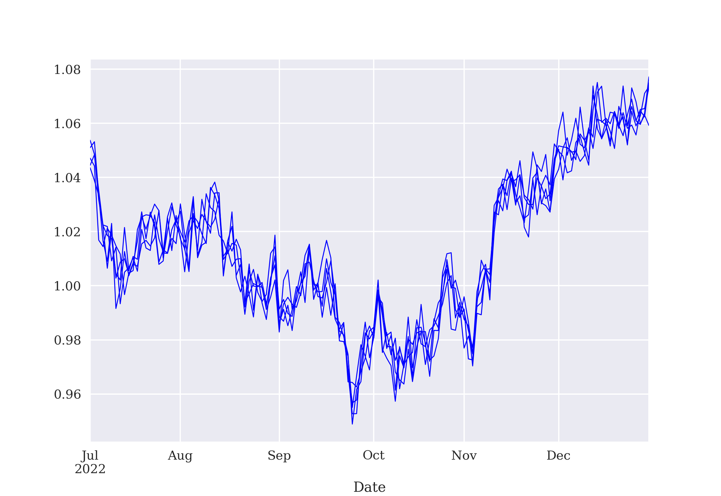

Figure 2. Noisy time series data for half a year

Using the new type of environment, the DQL agent — see the Python class in DQLAgent Python Class — can now be trained with a new, noisy data set for each episode. As the following Python code shows, the agent learns to distinguish between information (original movements) and the noisy components quite well:

In [16]: %run dqlagent.py

In [17]: os.environ['TF_CPP_MIN_LOG_LEVEL'] = '3'

In [18]: agent = DQLAgent(fin.symbol, fin.feature, fin.n_features, fin)

In [19]: %time agent.learn(250)
         episode= 250 | treward=   8.00 | max=1441.00
         CPU times: user 27.3 s, sys: 3.92 s, total: 31.2 s
         Wall time: 26.9 s

In [20]: agent.test(5)
         total reward=2604 | accuracy=0.601
         total reward=2604 | accuracy=0.590
         total reward=2604 | accuracy=0.597
         total reward=2604 | accuracy=0.593
         total reward=2604 | accuracy=0.617

4.2. Simulated Time Series Data

In Noisy Time Series Data, a historical financial time series is adjusted by adding white noise to it. In this section, the financial time series itself is simulated under suitable assumptions. Both approaches have in common that they allow the generation of an infinite number of different paths. However, using the Monte Carlo simulation (MCS) approach in this section leads to quite different paths in general that only on average show desired properties, such as a certain drift or a certain volatility.

In the following, a stochastic process according to Vasicek (1977) is simulated. Originally used to model the stochastic evolution of interest rates, it allows the simulation of trending or mean-reverting financial time series. The Vasicek model is described through the following stochastic differential equation^[16]:

\[dx_t = \kappa(\theta - x_t)dt+\sigma x_t dZ_t\]

Such processes are also called Ornstein-Uhlenbeck (OU) processes. The variables and parameters have the following meaning: $x_t$ is the process level at date t, $\kappa$ is the mean-reversion factor, $\theta$ is the long-term mean of the process, and $\sigma$ is the constant volatility parameter for $Z_t$ which is a standard Brownian motion.

For the simulations, a simple Euler discretization scheme is used (with $s = t - \Delta t$ and $z_t$ being standard normal):

\[x_t = x_s + \kappa(\theta - x_s)\Delta t + x_s \sigma \sqrt{\Delta t} z_t\]

The Simulation class implements a financial environment that relies on the simulation of the OU process above. The following Python code shows the initialization part of the class:

In [21]: class Simulation:
             def __init__(self, symbol, feature, n_features,
                          start, end, periods,
                          min_accuracy=0.525, x0=100,
                          kappa=1, theta=100, sigma=0.2,
                          normalize=True, new=False):
                 self.symbol = symbol
                 self.feature = feature
                 self.n_features = n_features
                 self.start = start  (1)
                 self.end = end  (2)
                 self.periods = periods  (3)
                 self.x0 = x0  (4)
                 self.kappa = kappa  (4)
                 self.theta = theta  (4)
                 self.sigma = sigma  (4)
                 self.min_accuracy = min_accuracy  (5)
                 self.normalize = normalize  (6)
                 self.new = new  (7)
                 self.action_space = ActionSpace()
                 self._simulate_data()
                 self._prepare_data()

1	The start date for the simulation.
2	The end date for the simulation
3	The number of periods to be simulated.
4	The OU model parameters for the simulation.
5	The minimum accuracy required to continue.
6	The parameter indicating whether normalization is applied to the data or not.
7	The parameter indicating whether a new simulation is initiated for every episode or not.

The following Python code shows the core method of the class. It implements the MCS for the OU process:

In [22]: import math
         class Simulation(Simulation):
             def _simulate_data(self):
                 index = pd.date_range(start=self.start,
                             end=self.end, periods=self.periods)
                 x = [self.x0]  (1)
                 dt = (index[-1] - index[0]).days / 365 / self.periods  (2)
                 for t in range(1, len(index)):
                     x_ = (x[t - 1] + self.kappa * (self.theta - x[t - 1]) * dt +
                           x[t - 1] * self.sigma * math.sqrt(dt) * random.gauss(0, 1))  (3)
                     x.append(x_)  (4)

                 self.data = pd.DataFrame(x, columns=[self.symbol], index=index)  (5)

1	The initial value of the process (boundary condition).
2	The length of the time interval, given the one-year horizon and the number of steps.
3	The Euler discretization scheme for the simulation itself.
4	The simulated value is appended to the `list` object.
5	The simulated process is transformed into a `DataFrame` object.

Data preparation is taken care of by the following code:

In [23]: class Simulation(Simulation):
             def _prepare_data(self):
                 self.data['r'] = np.log(self.data / self.data.shift(1))  (1)
                 self.data.dropna(inplace=True)
                 if self.normalize:
                     self.mu = self.data.mean()  (2)
                     self.std = self.data.std()  (2)
                     self.data_ = (self.data - self.mu) / self.std  (2)
                 else:
                     self.data_ = self.data.copy()
                 self.data['d'] = np.where(self.data['r'] > 0, 1, 0)  (3)
                 self.data['d'] = self.data['d'].astype(int)  (3)

1	Derives the log returns for the simulated process.
2	Applies Gaussian normalization to the data.
3	Derives the directional values from the log returns.

The following methods are helper methods and allow you, for example, to reset the environment:

In [24]: class Simulation(Simulation):
             def _get_state(self):
                 return self.data_[self.feature].iloc[self.bar -
                                         self.n_features:self.bar]  (1)
             def seed(self, seed):
                 random.seed(seed)  (2)
                 tf.random.set_seed(seed)  (2)
             def reset(self):
                 self.treward = 0
                 self.accuracy = 0
                 self.bar = self.n_features
                 if self.new:
                     self._simulate_data()
                     self._prepare_data()
                 state = self._get_state()
                 return state.values, {}

1	Returns the current set of feature values.
2	Fixes the seed for different random number generators.

The final method .step() is the same as for the NoisyData class:

In [25]: class Simulation(Simulation):
             def step(self, action):
                 if action == self.data['d'].iloc[self.bar]:
                     correct = True
                 else:
                     correct = False
                 reward = 1 if correct else 0
                 self.treward += reward
                 self.bar += 1
                 self.accuracy = self.treward / (self.bar - self.n_features)
                 if self.bar >= len(self.data):
                     done = True
                 elif reward == 1:
                     done = False
                 elif (self.accuracy < self.min_accuracy and self.bar > 25):
                     done = True
                 else:
                     done = False
                 next_state = self.data_[self.feature].iloc[
                     self.bar - self.n_features:self.bar].values
                 return next_state, reward, done, False, {}

With the complete Simulation class, different processes can be simulated. The next code snippet uses three different sets of parameters:

Baseline: No volatility or trending (long-term mean > initial value)
Trend: Volatility and trending (long-term mean > initial value)
Mean-reversion: Volatility and mean-reverting (long-term mean = initial value)

The simulated OU processes^[17] shows the simulated processes graphically.

In [26]: sym = 'EUR='

In [27]: env_base = Simulation(sym, sym, 5, start='2024-1-1', end='2025-1-1',
                          periods=252, x0=1, kappa=1, theta=1.1, sigma=0.0,
                          normalize=True)  (1)
         env_base.seed(100)

In [28]: env_trend = Simulation(sym, sym, 5, start='2024-1-1', end='2025-1-1',
                          periods=252, x0=1, kappa=1, theta=2, sigma=0.1,
                          normalize=True)  (2)
         env_trend.seed(100)

In [29]: env_mrev = Simulation(sym, sym, 5, start='2024-1-1', end='2025-1-1',
                          periods=252, x0=1, kappa=1, theta=1, sigma=0.1,
                          normalize=True)  (3)
         env_mrev.seed(100)

In [30]: env_mrev.data[sym].iloc[:3]
Out[30]: 2024-01-02 10:59:45.657370517    1.004236
         2024-01-03 21:59:31.314741035    1.009752
         2024-01-05 08:59:16.972111553    1.011010
         Name: EUR=, dtype: float64

In [31]: env_base.data[sym].plot(figsize=(10, 6), label='baseline', style='r')
         env_trend.data[sym].plot(label='trend', style='b:')
         env_mrev.data[sym].plot(label='mean-reversion', style='g--')
         plt.legend();

1	The baseline case.
2	The trend case.
3	The mean-reversion case.

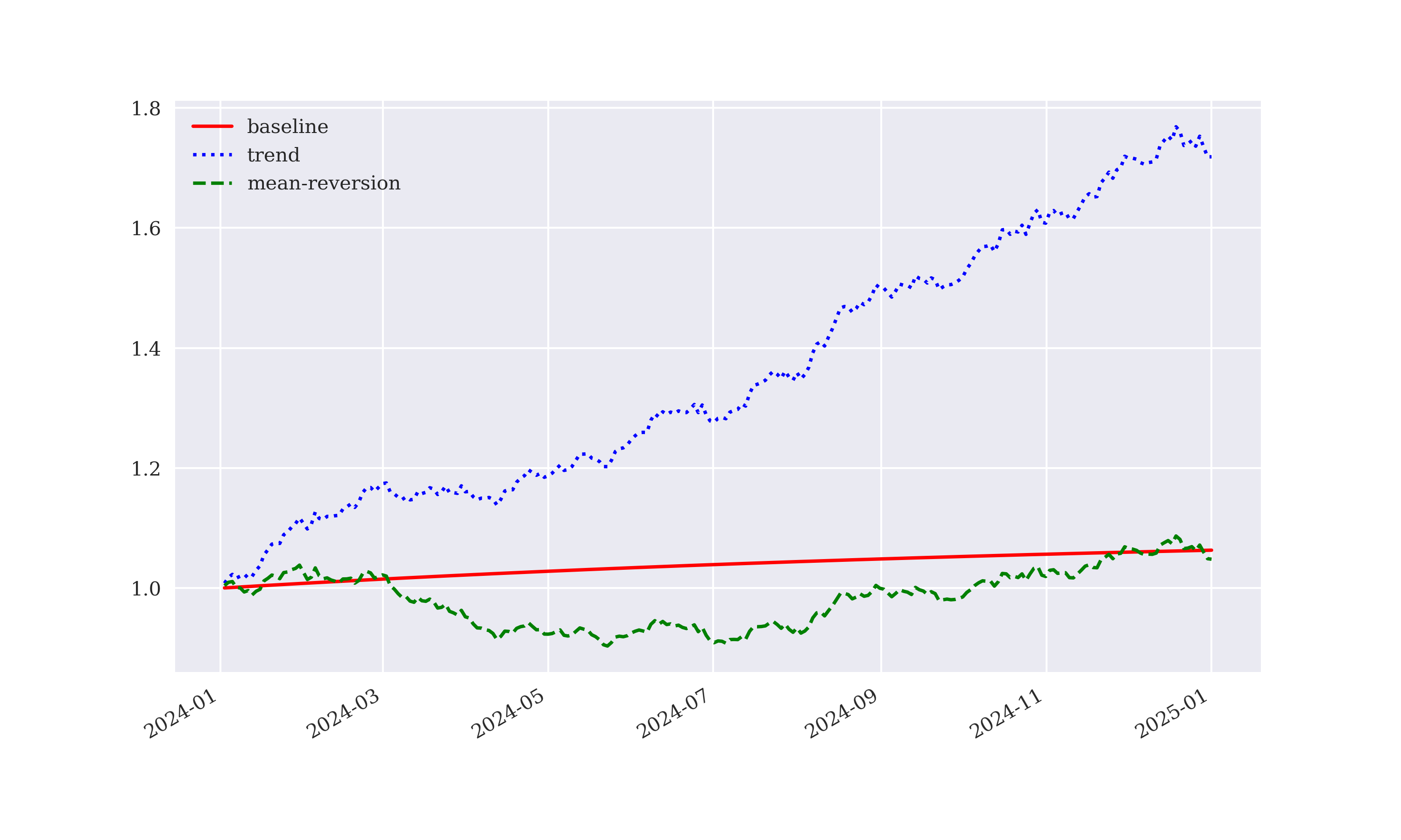
Figure 3. The simulated OU processes^[17]

Model Parameter Choice

The Vasicek (1977) model provides a certain degree of flexibility to simulate stochastic processes with different characteristics. However, in practical applications the parameters would not be chosen arbitrarily but rather derived — through optimization methods — from market observed data. This procedure is generally called model calibration and has a long tradition in computational finance. See, for example, Hilpisch (2015) for more details.

By default, resetting the Simulation environment generates a new simulated OU process, as Multiple simulated, trending OU processes illustrates.

In [32]: sim = Simulation(sym, 'r', 4, start='2024-1-1', end='2028-1-1',
                          periods=2 * 252, min_accuracy=0.485, x0=1,
                          kappa=2, theta=2, sigma=0.15,
                          normalize=True, new=True)
         sim.seed(100)

In [33]: for _ in range(10):
             sim.reset()
             sim.data[sym].plot(figsize=(10, 6), lw=1.0, c='b');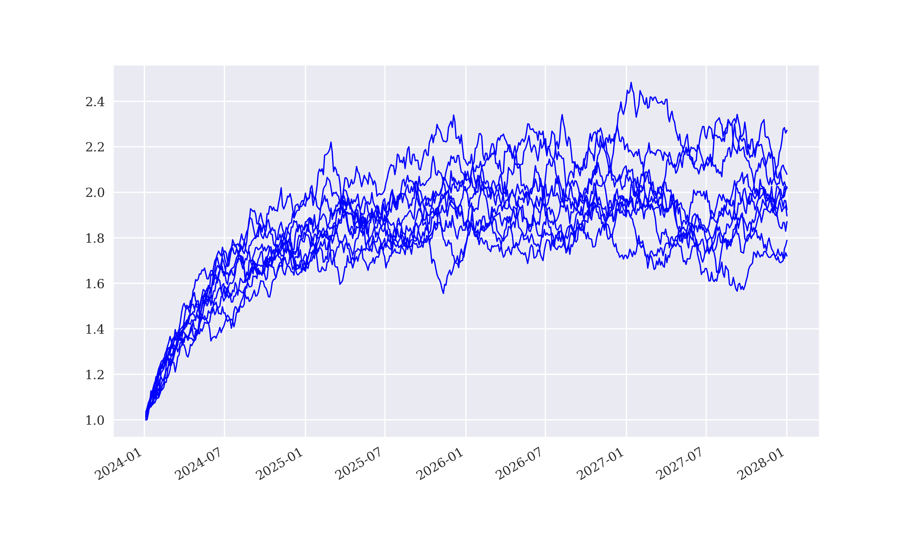

Figure 4. Multiple simulated, trending OU processes

The DQLAgent from DQLAgent Python Class works with this environment in the same way it worked with the NoisyData environment in the previous section. The following example uses the parametrization from before for the Simulation environment, which is a trending case. The agent learns quite well to predict the future directional movement:

In [34]: agent = DQLAgent(sim.symbol, sim.feature, sim.n_features, sim, lr=0.0001)

In [35]: %time agent.learn(500)
         episode= 500 | treward= 265.00 | max= 286.00
         CPU times: user 42.1 s, sys: 5.87 s, total: 47.9 s
         Wall time: 40.1 s

In [36]: agent.test(5)
         total reward= 499 | accuracy=0.547
         total reward= 499 | accuracy=0.515
         total reward= 499 | accuracy=0.561
         total reward= 499 | accuracy=0.533
         total reward= 499 | accuracy=0.549

The next example assumes a mean-reverting case, in which the DQLAgent is not able to predict the future directional movements as well as before. It seems that learning a trend might be easier than learning from simulated mean-reverting processes:

In [37]: sim = Simulation(sym, 'r', 4, start='2024-1-1', end='2028-1-1',
                          periods=2 * 252, min_accuracy=0.6, x0=1,
                          kappa=1.25, theta=1, sigma=0.15,
                          normalize=True, new=True)
         sim.seed(100)

In [38]: agent = DQLAgent(sim.symbol, sim.feature, sim.n_features, sim, lr=0.0001)

In [39]: %time agent.learn(500)
         episode= 500 | treward=  12.00 | max=  70.00
         CPU times: user 17.8 s, sys: 2.66 s, total: 20.4 s
         Wall time: 16.3 s

In [40]: agent.test(5)
         total reward= 499 | accuracy=0.487
         total reward= 499 | accuracy=0.495
         total reward= 499 | accuracy=0.511
         total reward= 499 | accuracy=0.487
         total reward= 499 | accuracy=0.449

4.3. Conclusions

The addition of white noise to a historical financial time series allows, in principle, the generation of an unlimited number of data sets to train a DQL agent. By varying the degree of noise, i.e. the standard deviation, the adjusted time series data might be close to or very different from the original time series. For the DQL agent, it can therefore be made easier or more difficult to learn to distinguish information from the added noise.

Simulation approaches were introduced to finance long before the wide-spread adoption of computers in the industry. Boyle (1977) is considered the seminal article in this regard. Glasserman (2004) provides a comprehensive overview of MCS techniques for finance.

Using MCS for OU processes allows the simulation of trending and mean-reverting processes. Typical trending financial time series are stock index levels or individual stock prices. Typical mean-reverting financial time series are FX rates or commodity prices.

In this chapter, the parameters for the simulation are assumed “out-of-the-blue”. In a more realistic setting, appropriate parameter values could be found, for example, through the calibration of the Vasicek (1977) model to the prices of liquidly traded options — an approach with a long tradition in computational finance.^[18]

The examples in this chapter show that the DQLAgent can more easily learn about trending time series than about mean-reverting ones. The next chapter turns the attention on generative approaches for the creation of synthetic time series data based on neural networks.

4.4. References

Books and articles cited in this chapter:

Boyle, Phelim (1977): “Options: A Monte Carlo Approach.” Journal of Financial Economics, Vol. 4, No. 4, pp. 322–338.
Glasserman, Paul (2004): Monte Carlo Methods in Financial Engineering. Springer, New York.
Halevy, Alon, Peter Norvig, and Fernando Preira (2009): “The Unreasonable Effectiveness of Data.” IEEE Intelligent Systems, March/April, 9-12.
Hilpisch, Yves (2018) Python for Finance—Mastering Data-Driven Finance. 2nd ed., O’Reilly, Sebastopol et al.
Hilpisch, Yves (2015): Derivatives Analytics with Python. Wiley Finance, Chichester.
Vasicek, Oldrich (1977). “An equilibrium characterization of the term structure.” Journal of Financial Economics, Vol. 5, No. 2, 177–188.

4.5. `DQLAgent` Python Class

The following Python code is from the dqlagent.py module and contains the DQLAgent class used in this chapter:

#
# Deep Q-Learning Agent
#
# (c) Dr. Yves J. Hilpisch
# Reinforcement Learning for Finance
#

import os
import random
import warnings
import numpy as np
import tensorflow as tf
from tensorflow import keras
from collections import deque
from keras.layers import Dense, Flatten
from keras.models import Sequential

warnings.simplefilter('ignore')
os.environ['TF_CPP_MIN_LOG_LEVEL'] = '3'


from tensorflow.python.framework.ops import disable_eager_execution
disable_eager_execution()

opt = keras.optimizers.legacy.Adam


class DQLAgent:
    def __init__(self, symbol, feature, n_features, env, hu=24, lr=0.001):
        self.epsilon = 1.0
        self.epsilon_decay = 0.9975
        self.epsilon_min = 0.1
        self.memory = deque(maxlen=2000)
        self.batch_size = 32
        self.gamma = 0.5
        self.trewards = list()
        self.max_treward = -np.inf
        self.n_features = n_features
        self.env = env
        self.episodes = 0
        self._create_model(hu, lr)
        
    def _create_model(self, hu, lr):
        self.model = Sequential()
        self.model.add(Dense(hu, activation='relu',
                             input_dim=self.n_features))
        self.model.add(Dense(hu, activation='relu'))
        self.model.add(Dense(2, activation='linear'))
        self.model.compile(loss='mse', optimizer=opt(learning_rate=lr))
        
    def _reshape(self, state):
        state = state.flatten()
        return np.reshape(state, [1, len(state)])
            
    def act(self, state):
        if random.random() < self.epsilon:
            return self.env.action_space.sample()
        return np.argmax(self.model.predict(state)[0])
        
    def replay(self):
        batch = random.sample(self.memory, self.batch_size)
        for state, action, next_state, reward, done in batch:
            if not done:
                reward += self.gamma * np.amax(
                    self.model.predict(next_state)[0])
                target = self.model.predict(state)
                target[0, action] = reward
                self.model.fit(state, target, epochs=1, verbose=False)
        if self.epsilon > self.epsilon_min:
            self.epsilon *= self.epsilon_decay
            
    def learn(self, episodes):
        for e in range(1, episodes + 1):
            self.episodes += 1
            state, _ = self.env.reset()
            state = self._reshape(state)
            treward = 0
            for f in range(1, 5000):
                self.f = f
                action = self.act(state)
                next_state, reward, done, trunc, _ = self.env.step(action)
                treward += reward
                next_state = self._reshape(next_state)
                self.memory.append(
                    [state, action, next_state, reward, done])
                state = next_state 
                if done:
                    self.trewards.append(treward)
                    self.max_treward = max(self.max_treward, treward)
                    templ = f'episode={self.episodes:4d} | '
                    templ += f'treward={treward:7.3f}'
                    templ += f' | max={self.max_treward:7.3f}'
                    print(templ, end='\r')
                    break
            if len(self.memory) > self.batch_size:
                self.replay()
        print()
        
    def test(self, episodes, min_accuracy=0.0,
             min_performance=0.0, verbose=True,
             full=True):
        ma = self.env.min_accuracy
        self.env.min_accuracy = min_accuracy
        if hasattr(self.env, 'min_performance'):
            mp = self.env.min_performance
            self.env.min_performance = min_performance
            self.performances = list()
        for e in range(1, episodes + 1):
            state, _ = self.env.reset()
            state = self._reshape(state)
            for f in range(1, 5001):
                action = np.argmax(self.model.predict(state)[0])
                state, reward, done, trunc, _ = self.env.step(action)
                state = self._reshape(state)
                if done:
                    templ = f'total reward={f:4d} | '
                    templ += f'accuracy={self.env.accuracy:.3f}'
                    if hasattr(self.env, 'min_performance'):
                        self.performances.append(self.env.performance)
                        templ += f' | performance={self.env.performance:.3f}'
                    if verbose:
                        if full:
                            print(templ)
                        else:
                            print(templ, end='\r')
                    break
        self.env.min_accuracy = ma
        if hasattr(self.env, 'min_performance'):
            self.env.min_performance = mp
        print()

5. Generated Data

In the proposed adversarial nets framework, the generative model is pitted against an adversary: a discriminative model that learns to determine whether a sample is from the model distribution or the data distribution. The generative model can be thought of as analogous to a team of counterfeiters, trying to produce fake currency and use it without detection, while the discriminative model is analogous to the police, trying to detect the counterfeit currency. Competition in this game drives both teams to improve their methods until the counterfeits are indistinguishable from the genuine articles.

— Goodfellow et al. (2014)

In their seminal paper Goodfellow et al. (2014), the authors introduce generative adversarial nets (GANs) that rely on a so-called generator and discriminator. The generator is trained on a given data set. Its purpose is to generate data that is similar “in nature”, that is, in a statistical sense, to the original data set. The discriminator is trained to distinguish between samples from the original data set and samples generated by the generator. The goal is to train the generator in a way that the discriminator cannot distinguish anymore between original samples and generated ones.

Although this approach might sound relatively simple at first, it has seen a large number of breakthrough applications after its publication. There are GANs available nowadays that create images, paintings, cartoons, text, poems, songs, computer code, and even videos that are hardly or even impossible to distinguish from human work. Between 2022 and 2024 alone, so many GANs have been published — open ones and commercial ones — that it is impossible to provide an exhaustive list.

GANs can also be used to create synthetic time series data that in turn can be used to train reinforcement learning agents. Similar to the noisy data and Monte Carlo simulation approaches of Simulated Data, GANs can generate a theoretically infinite set of synthetic time series.

The chapter proceeds as follows. Simple Example illustrates the training of a GAN based on data generated by a deterministic function. Financial Example then trains a GAN based on historical returns data of a financial instrument. The goal for the generator is to generate synthetic returns data that is, in the best case, indistinguishable for the discriminator from the real returns data. In addition, the Kolmogorow-Smirnow statistical test is applied to illustrate that synthetic returns data can also be indistinguishable from real data for traditional statistical tests.

5.1. Simple Example

This section deals with data generated by a deterministic mathematical function. First, some typical Python imports and configurations:

In [1]: import os
        import numpy as np
        import pandas as pd
        from pylab import plt, mpl

In [2]: import tensorflow as tf
        from tensorflow.keras.models import Sequential
        from tensorflow.keras.layers import Dense
        from tensorflow.keras.optimizers import Adam
        from sklearn.preprocessing import StandardScaler

In [3]: plt.style.use('seaborn-v0_8')
        mpl.rcParams['figure.dpi'] = 300
        mpl.rcParams['savefig.dpi'] = 300
        mpl.rcParams['font.family'] = 'serif'
        os.environ['TF_CPP_MIN_LOG_LEVEL'] = '3'

Second, the original data is generated from a simple mathematical function and is normalized. Real data (solid line), normalized data (dashed line) shows the two data sets as lines.

In [4]: x = np.linspace(-2, 2, 500)  (1)

In [5]: def f(x):
            return x ** 3  (2)

In [6]: y = f(x)  (3)

In [7]: scaler = StandardScaler()  (4)

In [8]: y_ = scaler.fit_transform(y.reshape(-1, 1))  (4)

In [9]: plt.plot(x, y, 'r', lw=1.0,
                 label='real data')
        plt.plot(x, y_, 'b--', lw=1.0,
                 label='normalized data')
        plt.legend();

1	Generates the input values of a given interval.
2	Defines the mathematical function (cubic monomial).
3	Generates the output values.
4	Normalizes the data using Gaussian normalization.

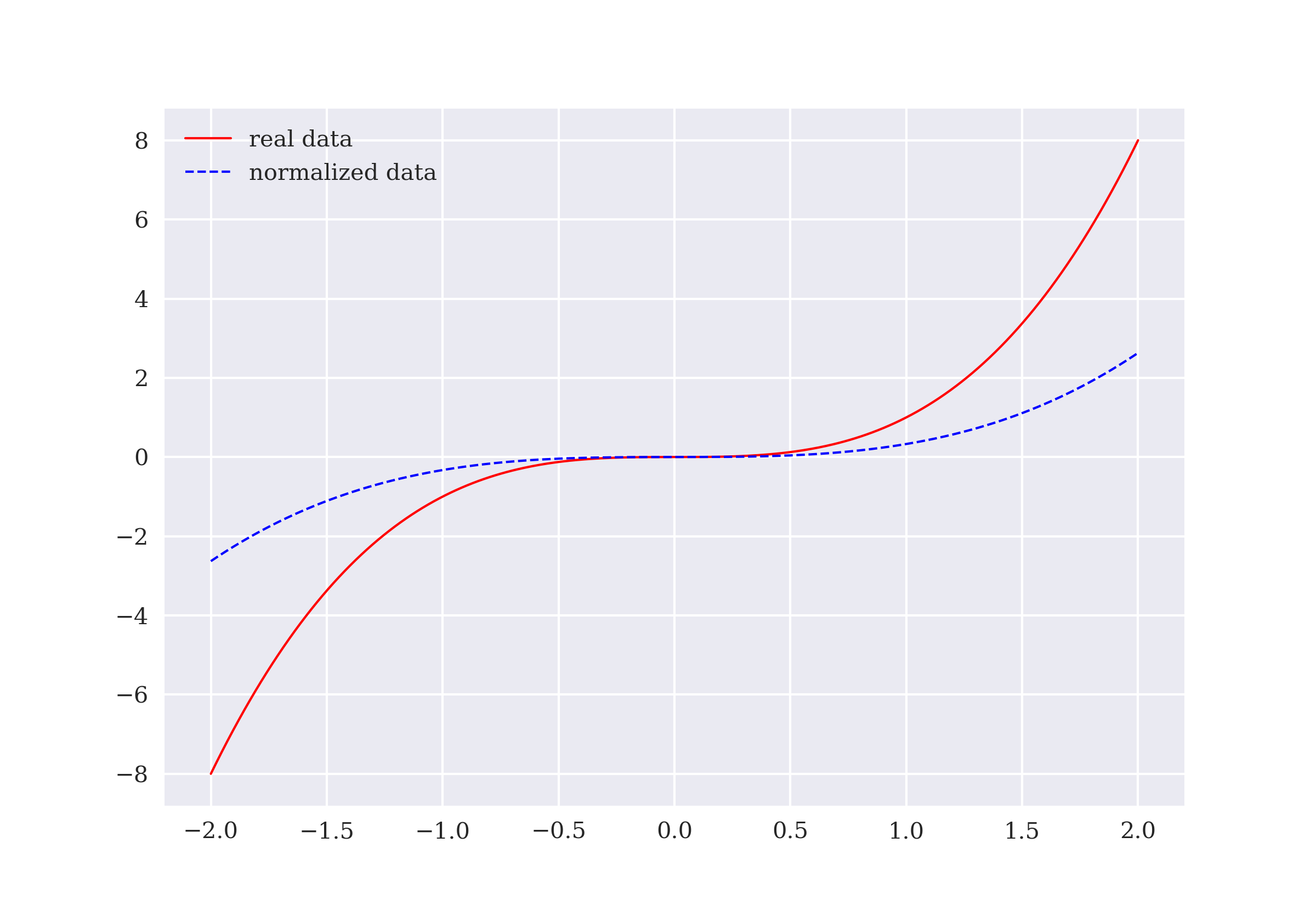
Figure 5. Real data (solid line), normalized data (dashed line)

The following Python code creates the first component of the GAN: the generator. It is a simple, standard dense neural network (DNN) for estimation:

In [10]: def create_generator(hu=32):
             model = Sequential()
             model.add(Dense(hu, activation='relu', input_dim=1))
             model.add(Dense(hu, activation='relu'))
             model.add(Dense(1, activation='linear'))
             return model

The second component of the GAN is the discriminator which is created through the following Python function. The model is again a simple, standard DNN — but this time for binary classification:

In [11]: def create_discriminator(hu=32):
             model = Sequential()
             model.add(Dense(hu, activation='relu', input_dim=1))
             model.add(Dense(hu, activation='relu'))
             model.add(Dense(1, activation='sigmoid'))
             model.compile(loss='binary_crossentropy', optimizer=Adam(),
                           metrics=['accuracy'])
             return model

The GAN is created by taking the generator and discriminator models as input arguments. For the GAN, the discriminator is set to “not trainable” — only the generator is trained with the GAN:

In [12]: def create_gan(generator, discriminator, lr=0.001):
             discriminator.trainable = False  (1)
             model = Sequential()
             model.add(generator)  (2)
             model.add(discriminator)  (3)
             model.compile(loss='binary_crossentropy',
                           optimizer=Adam(learning_rate=lr))
             return model

In [13]: generator = create_generator()  (4)
         discriminator = create_discriminator()  (4)
         gan = create_gan(generator, discriminator, 0.0001)  (4)

1	The discriminator model is not trained.
2	The generator model is added first to the GAN.
3	The discriminator model is added second to the GAN.
4	The three models are created in sequence.

With the three models created, the training of the models can take place. The following Python code trains the models over many epochs and a randomly sampled batch of a given size per epoch:

In [14]: from numpy.random import default_rng

In [15]: rng = default_rng(seed=100)

In [16]: def train_models(y_, epochs, batch_size):
             for epoch in range(epochs):
                 # Generate synthetic data
                 noise = rng.normal(0, 1, (batch_size, 1))  (1)
                 synthetic_data = generator.predict(noise, verbose=False)  (2)

                 # Train discriminator
                 real_data = y_[rng.integers(0, len(y_), batch_size)]  (3)
                 discriminator.train_on_batch(real_data, np.ones(batch_size))  (4)
                 discriminator.train_on_batch(synthetic_data,
                                              np.zeros(batch_size))  (5)

                 # Train generator
                 noise = rng.normal(0, 1, (batch_size, 1))  (6)
                 gan.train_on_batch(noise, np.ones(batch_size))  (7)

                 # Print progress
                 if epoch % 1000 == 0:
                     print(f'Epoch: {epoch}')
             return real_data, synthetic_data

In [17]: %%time
         real_data, synthetic_data = train_models(y_, epochs=5001, batch_size=32)
         Epoch: 0
         Epoch: 1000
         Epoch: 2000
         Epoch: 3000
         Epoch: 4000
         Epoch: 5000
         CPU times: user 1min 47s, sys: 10.9 s, total: 1min 58s
         Wall time: 1min 49s

1	Generates standard normally distributed noise …
2	… as input for the generator to create synthetic data.
3	Randomly samples data from the real data set.
4	Trains the discriminator on the real data sample (labels are 1).
5	Trains the discriminator on the synthetic data sample (labels are 0).
6	Generates standard normally distributed noise …
7	… as input for the training of the generator.

Normalized real and synthetic data sample shows the last real data and synthetic data samples from the training. These are the data sets the discriminator is confronted with. It is difficult to tell, just by visual inspection, whether the data sets are sampled from the real data or not. That feature is actually what the generator is striving for:

In [18]: plt.plot(real_data, 'r', lw=1.0, label='real data (last batch)')
         plt.plot(synthetic_data, 'b:', lw=1.0, label='synthetic data (last batch)')
         plt.legend();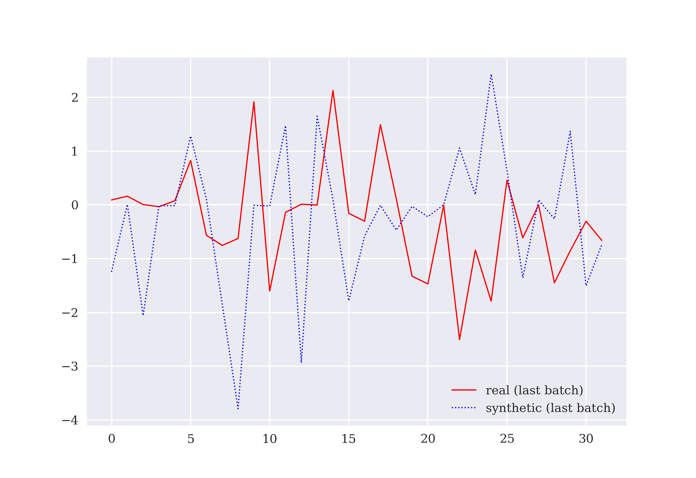

Figure 6. Normalized real and synthetic data sample

A more thorough analysis can shed more light on the statistical properties of the synthetic data sets generated by the GAN as compared to the real data from the mathematical function.

To this end, the following Python code generates several synthetic data sets of the length of the real data set. Several descriptive statistics, such as minimum, mean, and maximum values can shed light on the similarity of the synthetic data sets and the real data set. In addition, the normalization of the data is reversed. As we can see, the descriptive statistics of the real data set and the synthetic data sets are not too dissimilar:

In [19]: data = pd.DataFrame({'real': y}, index=x)

In [20]: N = 5  (1)
         for i in range(N):
             noise = rng.normal(0, 1, (len(y), 1))
             synthetic_data = generator.predict(noise, verbose=False)
             data[f'synth_{i:02d}'] = scaler.inverse_transform(synthetic_data)

In [21]: data.describe().round(3)
Out[21]:           real  synth_00  synth_01  synth_02  synth_03  synth_04
         count  500.000   500.000   500.000   500.000   500.000   500.000
         mean    -0.000    -0.110    -0.107    -0.311    -0.142    -0.128
         std      3.045     2.768     2.888     2.776     2.898     3.016
         min     -8.000   -12.046   -11.748   -10.252   -10.033    -8.818
         25%     -1.000    -0.890    -1.035    -1.241    -1.119    -1.193
         50%     -0.000    -0.031    -0.035    -0.048    -0.046    -0.041
         75%      1.000     0.862     0.884     0.546     0.731     0.746
         max      8.000     9.616    11.951     8.266     7.449     9.399

1	Five synthetic data sets of full length are generated.

The real data set is generated from a monotonically increasing function. Therefore, the following visualization shows the real data set and the synthetically generated data sets sorted, that is, in ascending order from the smallest to the largest value. As Real data (solid line) and sorted synthetic data sets (dashed lines) shows, the sorted synthetic data captures the basic shape of the real data quite well. It does it particularly well around 0. It does not do so well on the left and right limits of the interval. The similarity of the data sets is illustrated by the relatively low mean-squared error (MSE) for the first synthetic data set.

In [22]: ((data.apply(np.sort)['real'] -
           data.apply(np.sort)['synth_00']) ** 2).mean()  (1)
Out[22]: 0.22622928664937703

In [23]: data.apply(np.sort).plot(style=['r'] + N * ['b--'], lw=1, legend=False);

1	MSE for the sorted first synthetic data set, given the real data set.

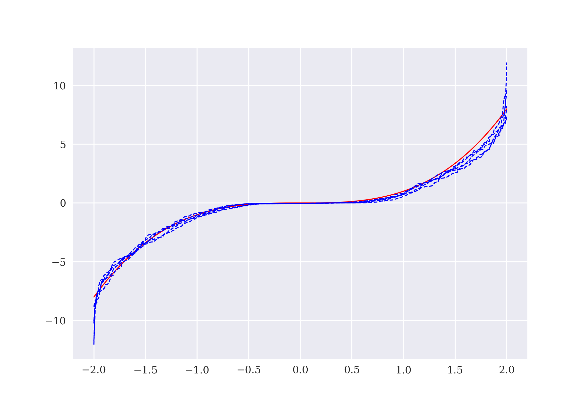
Figure 7. Real data (solid line) and sorted synthetic data sets (dashed lines)

5.2. Financial Example

This section applies the GAN approach from Simple Example to financial returns data. The goal for the generator is to generate synthetic returns data that the discriminator cannot distinguish from the real returns data. The Python code is essentially the same.

First, the financial data is retrieved and the log returns are calculated and normalized:

In [24]: raw = pd.read_csv('https://certificate.tpq.io/rl4finance.csv',
                          index_col=0, parse_dates=True).dropna()  (1)

In [25]: rets = raw['GLD'].iloc[-2 * 252:]  (2)
         rets = np.log((rets / rets.shift(1)).dropna())  (3)
         rets = rets.values  (4)

In [26]: scaler = StandardScaler()  (5)

In [27]: rets_ = scaler.fit_transform(rets.reshape(-1, 1))  (5)

1	Retrieves the financial data set from the remote source.
2	Selects, for a given symbol, a subset of the price data.
3	Calculates the log returns from the price data.
4	Transforms the `pandas Series` object into a `numpy ndarray` object.
5	Applies Gaussian normalization to the log returns.

Second, the creation of the three models: the generator, the discriminator, and the GAN itself:

In [28]: rng = default_rng(100)
         tf.random.set_seed(100)

In [29]: generator = create_generator(hu=24)
         discriminator = create_discriminator(hu=24)
         gan = create_gan(generator, discriminator, lr=0.0001)

Third, the training of the models:

In [30]: %time rd, sd = train_models(y_=rets_, epochs=5001, batch_size=32)
         Epoch: 0
         Epoch: 1000
         Epoch: 2000
         Epoch: 3000
         Epoch: 4000
         Epoch: 5000
         CPU times: user 1min 44s, sys: 10.6 s, total: 1min 55s
         Wall time: 1min 45s

Fourth, the generation of the synthetic data. Real and synthetic log returns shows the real log returns and one synthetic data set for comparison:

In [31]: data = pd.DataFrame({'real': rets})

In [32]: N = 25

In [33]: for i in range(N):
             noise = np.random.normal(0, 1, (len(rets_), 1))  (1)
             synthetic_data = generator.predict(noise, verbose=False)  (1)
             data[f'synth_{i:02d}'] = scaler.inverse_transform(synthetic_data)  (2)

In [34]: res = data.describe().round(4)  (3)
         res.iloc[:, :5]  (3)
Out[34]:            real  synth_00  synth_01  synth_02  synth_03
         count  503.0000  503.0000  503.0000  503.0000  503.0000
         mean     0.0002    0.0003    0.0007   -0.0001    0.0003
         std      0.0090    0.0088    0.0082    0.0084    0.0084
         min     -0.0302   -0.0269   -0.0385   -0.0277   -0.0246
         25%     -0.0052   -0.0052   -0.0044   -0.0054   -0.0046
         50%      0.0003   -0.0004    0.0007    0.0001    0.0008
         75%      0.0054    0.0059    0.0062    0.0045    0.0051
         max      0.0316    0.0263    0.0275    0.0321    0.0306

In [35]: data.iloc[:, :2].plot(style=['r', 'b--', 'b--'], lw=1, alpha=0.7);

1	Generates random synthetic data.
2	Inverse transforms the data and stores it.
3	Shows descriptive statistics for real and synthetic data.

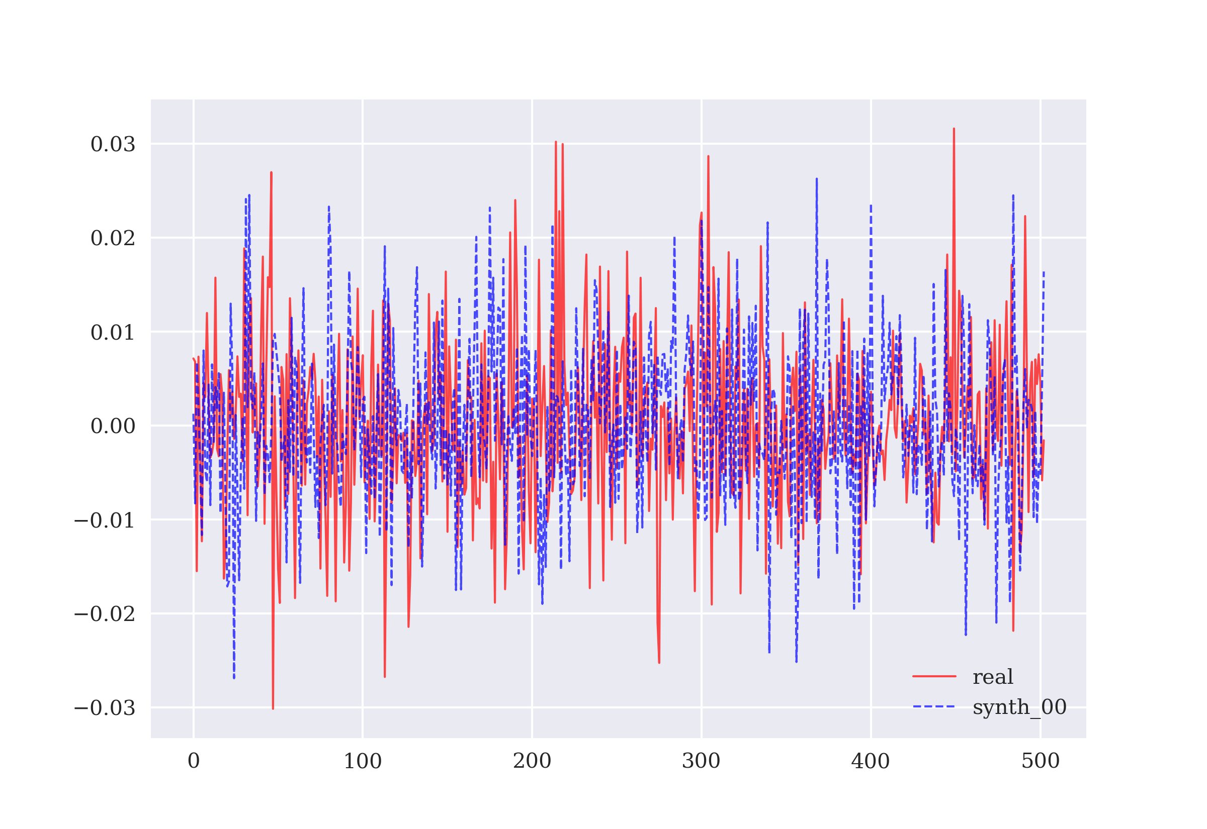
Figure 8. Real and synthetic log returns

The following Python code compares the real and synthetic log returns based on their histograms (see Histogram of the real and synthetic log returns). The histograms show a large degree of similarity:

In [36]: data['real'].plot(kind='hist', bins=50, label='real',
                           color='r', alpha=0.7)
         data['synth_00'].plot(kind='hist', bins=50, alpha=0.7,
                           label='synthetic', color='b', sharex=True)
         plt.legend();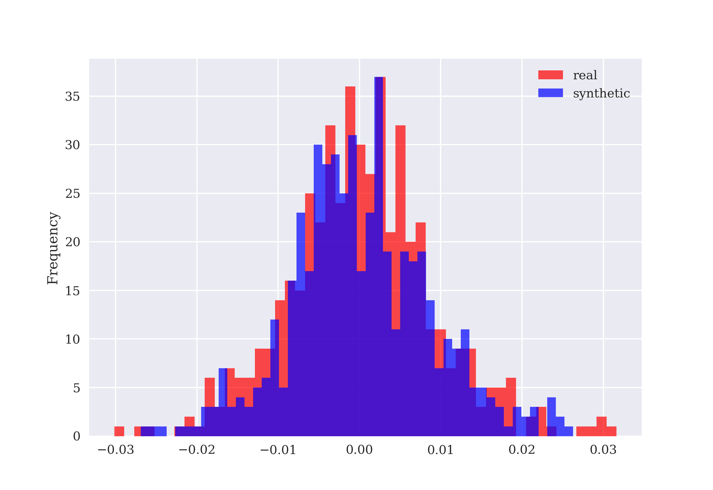

Figure 9. Histogram of the real and synthetic log returns

CDF of the real and synthetic log returns provides yet another comparison, this time based on the empirical cumulative distribution function (CDF) of the real and the synthetic log returns:

In [37]: plt.plot(np.sort(data['real']), 'r', lw=1.0, label='real')
         plt.plot(np.sort(data['synth_00']), 'b--', lw=1.0, label='synthetic')
         plt.legend();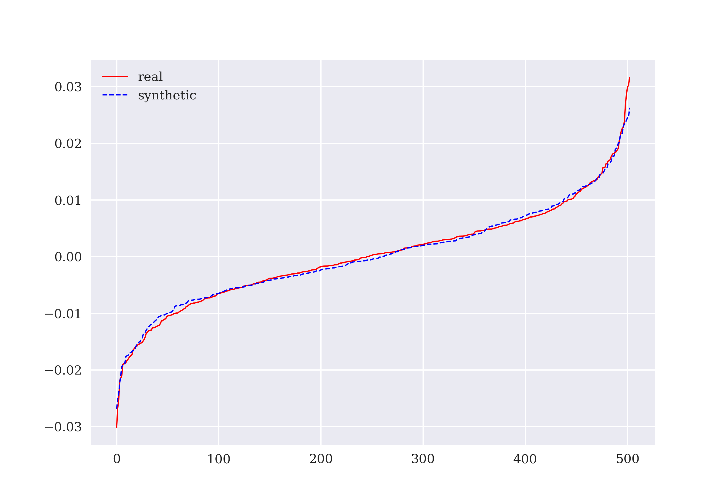

Figure 10. CDF of the real and synthetic log returns

Finally, the following Python code visualizes the cumulative real gross returns as well as several synthetic cumulative log return time series. The real financial time series looks like one that is generated with the GAN. Without the visual highlighting, it might indeed be indistinguishable from the other processes (see Real and synthetic cumulative log returns series).

In [38]: sn = N
         data.iloc[:, 1:sn + 1].cumsum().apply(np.exp).plot(
             style='b--', lw=0.7, legend=False)
         data.iloc[:, 1:sn + 1].mean(axis=1).cumsum().apply(
             np.exp).plot(style='g', lw=2)
         data['real'].cumsum().apply(np.exp).plot(style='r', lw=2);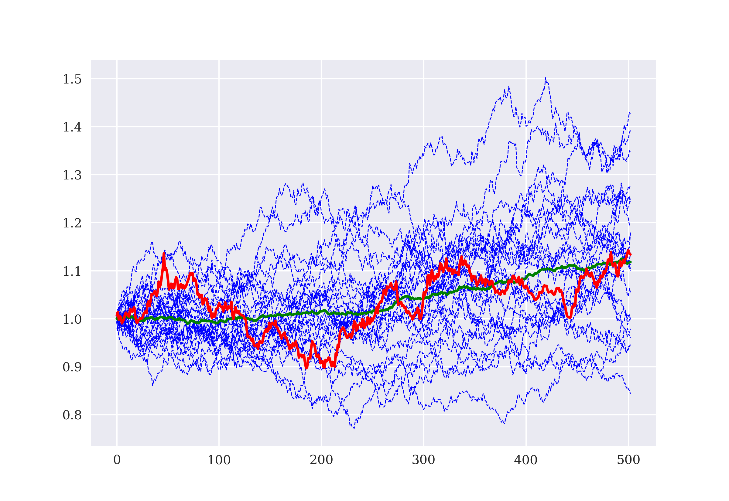

Figure 11. Real and synthetic cumulative log returns series

5.3. Kolmogorov-Smirnov Test

The Kolmogorov-Smirnov (KS) test is a statistical test that answers the following question: “How likely is it that a given data sample has been drawn from a given distribution?”.^[19] This description applies quite well to the situation in this chapter. A frequency distribution of the historical returns of a financial instrument is given, and it is the starting point for everything. A GAN is trained based on these historical returns. The GAN then generates multiple return samples synthetically. The question is how likely is it — applying the KS test — whether a given synthetic sample is drawn from the original distribution of historically observed returns? In other words, can the generator not only fool the discriminator but also the KS test?

The following Python code implements the KS test on the synthetically generated data samples. The results show that the KS test indicates in all cases that the sample is likely from the original distribution. Histogram of $p-$values of KS test shows the frequency distribution of the $p-$values of the KS test. All $p-$values are above the threshold value of 0.05 (vertical line) — in many instances, the values are significantly larger than the threshold value. The GAN seems to do a great job of fooling the KS test into indicating that the synthetic samples are from the original distribution.

In [39]: from scipy import stats

In [40]: pvs = list()
         for i in range(N):
             pvs.append(stats.kstest(data[f'synth_{i:02d}'], data['real']).pvalue)
         pvs = np.array(pvs)

In [41]: np.sort((pvs > 0.05).astype(int))
Out[41]: array([1, 1, 1, 1, 1, 1, 1, 1, 1, 1, 1, 1, 1, 1, 1, 1, 1, 1, 1, 1, 1,
          1,
                1, 1, 1])

In [44]: sum(np.sort(pvs > 0.05)) / N
Out[44]: 1.0

In [43]: plt.hist(pvs, bins=100)
         plt.axvline(0.05, color='r');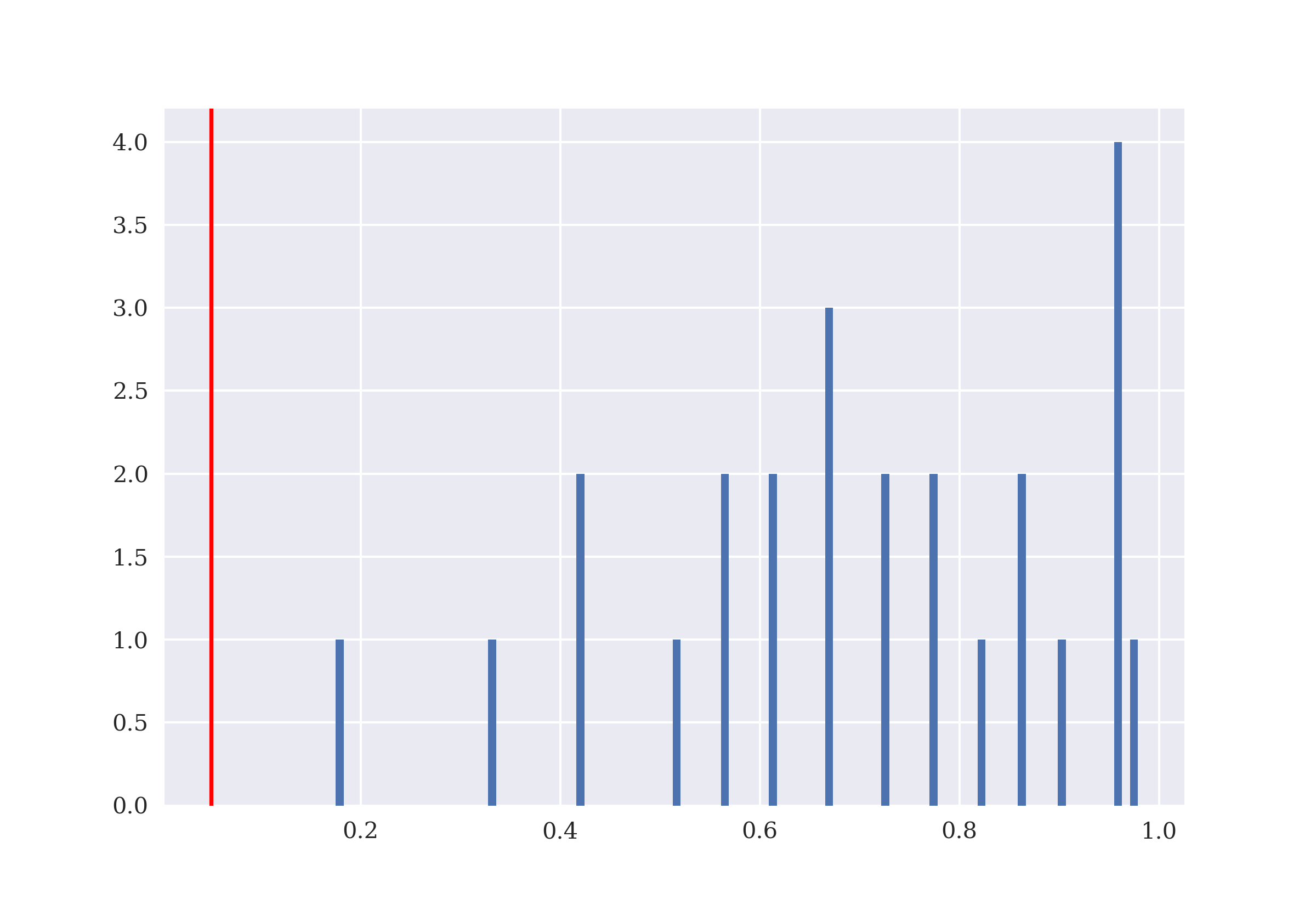

Figure 12. Histogram of $p-$values of KS test

The Power of GANs

The GAN approach to generating synthetic time series data seems to be a great one. Visualizations generally do not allow a human observer to distinguish between real data and synthetic. Nor is a DNN, that is, the discriminator, capable of properly distinguishing between the data sets. In addition, as this section shows, traditional and widely used statistical tests also fail to properly distinguish between real and synthetic data. For RL learning projects, GANs therefore seem to provide one option to generate theoretically infinite synthetic data sets that have all the qualities of the original data set of interest.

5.4. Conclusions

Neural networks can be trained to generate data that is similar to, or even indistinguishable from, real financial data. This chapter introduces GANs based on simple sample data generated from a deterministic mathematical function. It then shows how to apply the same GAN architecture to log returns from a real financial time series. The result is the availability of a theoretically infinite number of generated financial time series that can be used in RL or other financial applications. Creswell et al. (2017) provide an early overview of GANs while Eckerli and Osterrieder (2021) do so particularly for GANs in finance.

At first sight, GANs seem to do something very similar to the Monte Carlo simulation approach from Simulated Data. However, there are major differences. Monte Carlo simulation in general relies on a relatively simple, parsimonious mathematical model. A few parameters can be chosen to reflect certain statistical facts of the real financial time series to be simulated. One such approach is the calibration of the model parameters to the prices of liquidly traded options on the financial instrument whose price series is to be simulated.^[20]

On the other hand, GANs learn about the full distribution, say, of the log returns to be generated synthetically. The training of the generator DNN happens in competition with the discriminator DNN so the generator is getting better and better in mimicking the historical distribution. At the same time, the discriminator improves in distinguishing between real samples and synthetic samples of the log returns. Both DNNs are expected to improve during training to achieve good results overall.

The next part and the following chapters are about the application of the DQL algorithm to typical dynamic financial problems. They leverage the methods as introduced in this part to provide as many data samples for training and testing of the DQL agents as necessary.

5.5. References

Books and articles cited in this chapter:

Ecerkli, Florian and Joerg Osterrieder (2021): “Generative Adversarial Networks in Finance: An Overview.” https://ssrn.com/abstract=3864965.
Creswell, Antonia et al. (2017): “Generative Adversarial Networks: An Overview.” https://arxiv.org/abs/1710.07035.
Goodfellow, Ian et al. (2014): “Generative Adversarial Nets.” https://arxiv.org/abs/1406.2661.
Hilpisch, Yves (2015): Derivatives Analytics with Python—Data Analysis, Models, Simulation, Calibration and Hedging. John Wiley & Sons, Chichester.
Kolmogorov, Andrey (1933): “Sulla Determinazione Empirica di una Legge di Distribuzione.” Giornale dell’Istituto Italiano degli Attuari, Vol. 4, 83–91.

Financial Applications

The third part of the book applies the algorithms and techniques introduced in the first two parts to classical financial problems:

Algorithmic Trading applies deep Q-learning (DQL) to the algorithmic trading of a single financial instrument. It builds on the prediction game discussed in Financial Q-Learning. The chapter uses Monte Carlo simulated data to train a financial Q-learning agent, called TradingAgent. The goal of the FQL agent is to maximize the profit from going long and short on a single financial instrument.
Dynamic Hedging used DQL to learn how to hedge, or rather replicate, a European call option in the seminal model by Black-Scholes-Merton (1973) for option pricing. The HedgingAgent is able to learn appropriate hedging strategies by working with market-observable data only. For example, the agent knows the current price of the underlying, the time-to-maturity, and the current option price.
Dynamic Asset Allocation applies reinforcement learning (RL) to two problems in investment management. The first is to derive the optimal fraction of a portfolio to be bet on a financial instrument. This problem is usually addressed by applying the Kelly criterion. The InvestingAgent recovers the optimal Kelly fraction through maximization of the compound annual growth rate of the investment. The second problem is about the optimal portfolio composition for two negatively correlated assets. There are strong stylized facts that a constant proportion portfolio of the S&P 500 index (through an ETF or futures) and the VIX volatility index (through futures or options) outperforms alternative asset allocation schemes. The InvestingAgent is also able to recover this type of strategy through RL.

6. Algorithmic Trading

Automated stock-trading systems are widely used by major investing houses. While some of these are simply ways of automating the execution of particular buy or sell orders issued by a human fund manager, others pursue complicated trading strategies that adapt to changing market conditions.

— Bostrom (2014)

Financial giants such as Goldman Sachs and many of the biggest hedge funds are all switching on AI-driven systems that can foresee market trends and make trades better than humans.

— Maney (2017)

In Financial Q-Learning, the deep Q-learning (DQL) agent learns to predict the future direction of the price movement of a financial instrument. We have called this a financial prediction game. It is a natural progression to interpret the prediction game as a DQL agent learning to algorithmically trade in financial markets. A prediction of an upward movement can be interpreted as taking on a long position in the financial instrument of interest. Analogously, the prediction of a downward movement is interpreted as taking on a short position. Over time, the predictions might also imply keeping the current position open.

In addition to this reinterpretation of the prediction game as algorithmic trading, the financial side needs to be added. Taking on a long or short position in a financial instrument leads to a positive or negative return on such a position. Therefore, to assess the financial performance of the algorithmically trading DQL agent, its positions must be linked to their returns, specifically evaluating its accumulated profit and loss (P&L).

This chapter proceeds as follows. Prediction Game Revisited revisits the prediction game from Financial Q-Learning and the Finance environment developed there. It also uses the Simulation environment from Simulated Time Series Data to replace the single, fixed historical time series from the Finance class with an arbitrarily large number of simulated time series. Trading Environment introduces a trading environment that simulates the evolution of the price of a financial instrument along the lines of Simulated Time Series Data. The environment allows the selection of additional financial features in addition to the price itself and the log returns. Trading Agent trains the financial Q-learning (FQL) agent, called TradingAgent, on simulated data and tests for the financial performance of the trained agent in comparison to a randomly investing one.

6.1. Prediction Game Revisited

This section revisits the financial prediction game from Financial Q-Learning. To simplify the exposition, the Finance environment is imported from a Python module (see Finance Environment) as is the DQLAgent class (see DQLAgent Class). The DQLAgent class is changed in multiple instances. The major goal is to have the original DQLAgent class as a special case and to allow at the same time for multiple features instead of just one. First, the usual imports:

In [1]: import math
        import random
        import numpy as np
        import pandas as pd
        from pylab import plt, mpl

In [2]: plt.style.use('seaborn-v0_8')
        mpl.rcParams['figure.dpi'] = 300
        mpl.rcParams['savefig.dpi'] = 300
        mpl.rcParams['font.family'] = 'serif'
        np.set_printoptions(suppress=True)

The following Python code imports the Finance class and visualizes the time series of the price for the symbol chosen (see Historical financial time series data):

In [3]: from finance import *

In [4]: finance = Finance('GLD', 'r', min_accuracy=47.5,
                      n_features=8)

In [5]: finance.data[finance.symbol].plot(title=finance.symbol,
                                          lw=1.0, c='b');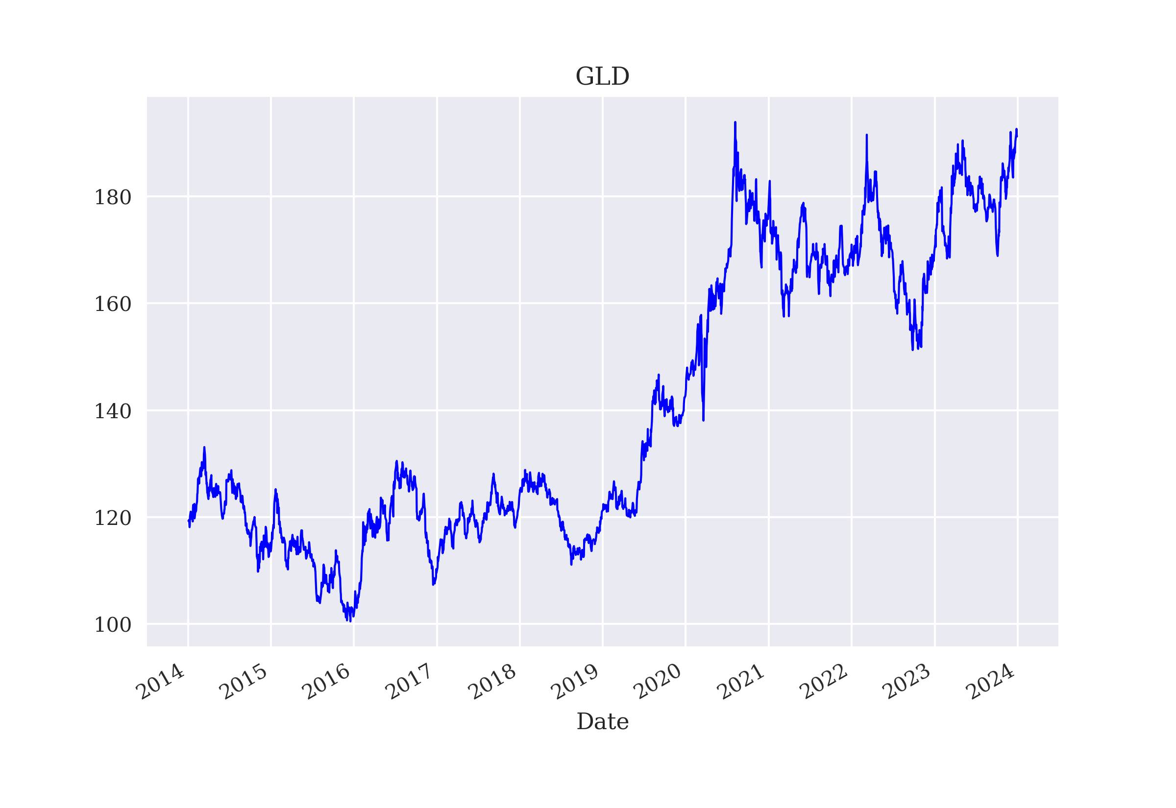

Figure 13. Historical financial time series data

With the finance environment object instantiated, a DQL agent can do its work. The following Python code trains the agent and implements a small number of tests. During the tests, a minimum threshold accuracy of 0 is assumed so that the agent will always reach the end of the data. The achieved accuracy does not vary because the data set is fixed and the agent only exploits its acquired knowledge as embodied in its neural network:

In [6]: from dqlagent import *

In [7]: random.seed(100)
        tf.random.set_seed(100)

In [8]: dqlagent = DQLAgent(finance.symbol, finance.feature,
                         finance.n_features, finance, lr=0.0001)

In [9]: %time dqlagent.learn(500)
        episode= 500 | treward=   8.00 | max=  12.00
        CPU times: user 14.5 s, sys: 1.96 s, total: 16.4 s
        Wall time: 13.2 s

In [10]: dqlagent.test(3)
         total reward=2507 | accuracy=0.516
         total reward=2507 | accuracy=0.516
         total reward=2507 | accuracy=0.516

The same DQL agent can also interact by default with the Simulation environment from Simulated Time Series Data. That class is imported from yet another Python module (see Simulation Environment). The chosen parametrization leads to a negatively trending time series as Simulated, trending financial time series data illustrates.

In [11]: from simulation import Simulation

In [12]: random.seed(500)

In [13]: simulation = Simulation('SYMBOL', 'r', 4, '2025-1-1', '2027-1-1', 2 * 252,
                          min_accuracy=0.5, x0=1, kappa=1, theta=0.75, sigma=0.1,
                          new=True, normalize=True)

In [14]: for _ in range(5):
             simulation.reset()
             simulation.data[simulation.symbol].plot(title=simulation.symbol,
                                                    lw=1.0, c='b');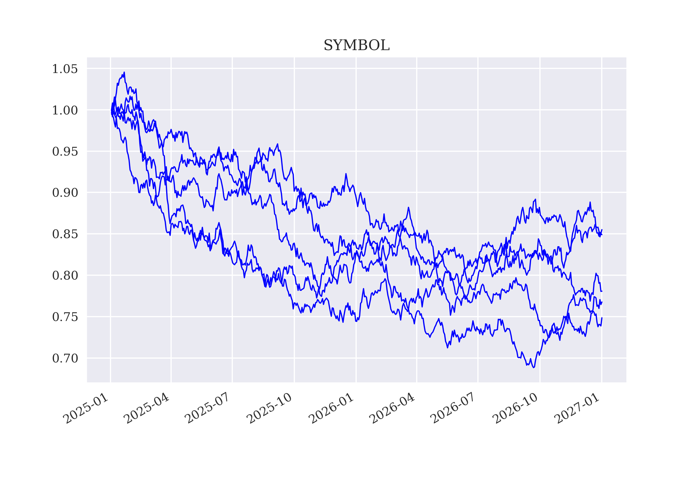

Figure 14. Simulated, trending financial time series data

This time, the DQL agent is faced with a new, simulated time series during every learning episode. The same holds for the testing runs so that the accuracy varies for every such run:

In [15]: random.seed(100)
         tf.random.set_seed(100)

In [16]: agent = DQLAgent(simulation.symbol, simulation.feature,
                          simulation.n_features, simulation)

In [17]: %time agent.learn(250)
         episode= 250 | treward=  16.00 | max= 279.00
         CPU times: user 10.8 s, sys: 1.61 s, total: 12.4 s
         Wall time: 10.1 s

In [18]: agent.test(5)
         total reward= 499 | accuracy=0.517
         total reward= 499 | accuracy=0.581
         total reward= 499 | accuracy=0.523
         total reward= 499 | accuracy=0.519
         total reward= 499 | accuracy=0.515

Both the Simulation environment and the DQLAgent class are modified in the subsequent sections. The major adjustments relate to the environment which shall provide a richer set of state variables than the Simulation one.

6.2. Trading Environment

Simulated Time Series Data introduces Monte Carlo simulation as a method to generate a theoretically infinite number of different time series with certain characteristics, such as trending or mean-reverting. The previous section revisits the prediction game context as set out in Financial Q-Learning against the background of such simulated time series data.

This section develops a new, yet similar, environment leveraging the Monte Carlo simulation approach and deriving several financial features from the simulated data. The environment allows an agent to retrieve multiple such features with a specified number of lags as the state of the environment. This approach enriches the state of the environment significantly as compared to the Simulation class from Simulated Time Series Data to improve the prediction capabilities of the DQL agent.

To keep things simple and in line with the RL approach implemented in Financial Q-Learning, the DQL agent is supposed to choose, as before, one of two possible actions. They are interpreted as taking a long position or a short position in the financial instrument whose price is simulated.

The following Python code provides the initialization method of the Trading class. This class requires a minimum accuracy for the prediction and a minimum financial performance during the training episodes. It also allows for leverage as this is typical, for example, in FX trading:

In [19]: class ActionSpace:
             def sample(self):
                 return random.randint(0, 1)

In [20]: class Trading:
             def __init__(self, symbol, features, window, lags,
                          start, end, periods,
                          x0=100, kappa=1, theta=100, sigma=0.2,
                          leverage=1, min_accuracy=0.5, min_performance=0.85,
                          mu=None, std=None,
                          new=True, normalize=True):
                 self.symbol = symbol
                 self.features = features
                 self.n_features = len(features)
                 self.window = window
                 self.lags = lags
                 self.start = start
                 self.end = end
                 self.periods = periods
                 self.x0 = x0
                 self.kappa = kappa
                 self.theta = theta
                 self.sigma = sigma
                 self.leverage = leverage  (1)
                 self.min_accuracy = min_accuracy  (2)
                 self.min_performance = min_performance  (3)
                 self.start = start
                 self.end = end
                 self.mu = mu
                 self.std = std
                 self.new = new
                 self.normalize = normalize
                 self.action_space = ActionSpace()
                 self._simulate_data()
                 self._prepare_data()

1	Defines the `leverage` attribute (`1` by default).
2	Defines the minimum prediction accuracy.
3	Defines the minimum performance in terms of gross performance.

The simulation of the time series data is again implemented as a discrete Vasicek (1977) Ornstein-Uhlenbeck process:

In [21]: class Trading(Trading):
             def _simulate_data(self):
                 index = pd.date_range(start=self.start,
                             end=self.end, periods=self.periods)
                 s = [self.x0]
                 dt = (index[-1] - index[0]).days / 365 / self.periods
                 for t in range(1, len(index)):
                     s_ = (s[t - 1] + self.kappa * (self.theta - s[t - 1]) * dt +
                       s[t - 1] * self.sigma * math.sqrt(dt) * random.gauss(0, 1))
                     s.append(s_)
                 self.data = pd.DataFrame(s, columns=[self.symbol], index=index)

The data preparation is where the new Trading class differs most from the original Simulation class. In addition to deriving the log returns, and based on these the market direction, the class adds several typical financial statistics to the set of available features. Among them are: a simple moving average (SMA), the rolling delta between the price and the SMA (DEL), the rolling minimum and maximum of the price (MIN, MAX), and the momentum as the rolling average return (MOM):

In [22]: class Trading(Trading):
             def _prepare_data(self):
                 self.data['r'] = np.log(self.data / self.data.shift(1))
                 self.data.dropna(inplace=True)
                 # additional features
                 if self.window > 0:
                     self.data['SMA'] = self.data[
                         self.symbol].rolling(self.window).mean()  (1)
                     self.data['DEL'] = self.data[
                         self.symbol] - self.data['SMA']  (2)
                     self.data['MIN'] = self.data[
                         self.symbol].rolling(self.window).min()  (3)
                     self.data['MAX'] = self.data[
                         self.symbol].rolling(self.window).max()  (4)
                     self.data['MOM'] = self.data['r'].rolling(
                         self.window).mean()  (5)
                     # add more features here
                     self.data.dropna(inplace=True)
                 if self.normalize:
                     if self.mu is None or self.std is None:
                         self.mu = self.data.mean()
                         self.std = self.data.std()
                     self.data_ = (self.data - self.mu) / self.std
                 else:
                     self.data_ = self.data.copy()
                 self.data['d'] = np.where(self.data['r'] > 0, 1, 0)
                 self.data['d'] = self.data['d'].astype(int)

1	Simple moving average (`SMA`) of the price.
2	Difference (`DEL`) between current price and the SMA.
3	Rolling minimum of the price (`MIN`).
4	Rolling maximum of the price (`MAX`).
5	Momentum as the rolling mean of the log return (`MOM`).

Adding Financial Features

The Trading class creates and works with several financial features. These are features that are regularly used by traders and investors who analyze financial price charts. However, there is a much larger number of such features available that can be added to the environment class.^[21] This might, depending on the use case, significantly improve the learning and performance of the DQL agent. While the state of a chess environment is definitively given at any time, the definition of the state of a financial market generally requires research, modeling effort, and testing to achieve satisfactory results with RL.

The following three methods are known from the Simulation class:

In [23]: class Trading(Trading):
             def _get_state(self):
                 return self.data_[self.features].iloc[self.bar -
                                         self.lags:self.bar]
             def seed(self, seed):
                 random.seed(seed)
                 np.random.seed(seed)
                 tf.random.set_random_seed(seed)
             def reset(self):
                 if self.new:
                     self._simulate_data()
                     self._prepare_data()
                 self.treward = 0
                 self.accuracy = 0
                 self.actions = list()
                 self.returns = list()
                 self.performance = 1
                 self.bar = self.lags
                 state = self._get_state()
                 return state.values, {}

The major difference in the .step() method is that it checks for the minimum required performance. This happens, like for the accuracy check, with a grace period of a certain number of bars:

In [24]: class Trading(Trading):
             def step(self, action):
                 correct = action == self.data['d'].iloc[self.bar]
                 ret = self.data['r'].iloc[self.bar] * self.leverage
                 reward_ = 1 if correct else 0
                 pl = abs(ret) if correct else -abs(ret)  (1)
                 reward = reward_
                 # alternative options:
                 # reward = pl  # only the P&L in log returns
                 # reward = reward_ + 10 * pl  # the reward + the scaled P&L
                 self.treward += reward
                 self.bar += 1
                 self.accuracy = self.treward / (self.bar - self.lags)
                 self.performance *= math.exp(pl)  (2)
                 if self.bar >= len(self.data):
                     done = True
                 elif reward_ == 1:
                     done = False
                 elif (self.accuracy < self.min_accuracy and
                       self.bar > self.lags + 15):
                     done = True
                 elif (self.performance < self.min_performance and
                       self.bar > self.lags + 15):  (3)
                     done = True
                 else:
                     done = False
                 state = self._get_state()
                 return state.values, reward, done, False, {}

1	Captures the log return for the trade.
2	Updates the performance given the realized log return.
3	Checks for the minimum performance criterion.

The following Python code instantiates a Trading object and shows the simulated and derived data, both selectively in numbers as well as visually (see Simulated financial time series data with multiple features). The Trading environment is closer to what traders and investors would typically analyze on their financial terminals and trading screens:

In [25]: symbol = 'SYMBOL'

In [26]: trading = Trading(symbol, [symbol, 'r', 'DEL'], window=10, lags=5,
                     start='2024-1-1', end='2026-1-1', periods=504,
                     x0=100, kappa=2, theta=300, sigma=0.1, normalize=False)

In [27]: random.seed(750)

In [28]: trading.reset()  (1)
Out[28]: (array([[115.90591443,   0.01926915,   6.89239862],
                 [117.17850569,   0.01091968,   6.5901155 ],
                 [118.79489427,   0.01369997,   6.65876779],
                 [120.63380354,   0.01536111,   6.92684742],
                 [121.81132396,   0.00971378,   6.65768164]]),
          {})

In [29]: trading.data.info()
         <class 'pandas.core.frame.DataFrame'>
         DatetimeIndex: 494 entries, 2024-01-15 12:47:14.194831014 to 2026-01-01
          00:00:00
         Data columns (total 8 columns):
          #   Column  Non-Null Count  Dtype
         ---  ------  --------------  -----
          0   SYMBOL  494 non-null    float64
          1   r       494 non-null    float64
          2   SMA     494 non-null    float64
          3   DEL     494 non-null    float64
          4   MIN     494 non-null    float64
          5   MAX     494 non-null    float64
          6   MOM     494 non-null    float64
          7   d       494 non-null    int64
         dtypes: float64(7), int64(1)
         memory usage: 34.7 KB

In [30]: trading.data.iloc[-200:][
             [trading.symbol, 'SMA', 'MIN', 'MAX']].plot(
                 style=['b-', 'r--', 'g:', 'g:'], lw=1.0);

1	The state consists now of multiple features with multiple lags.

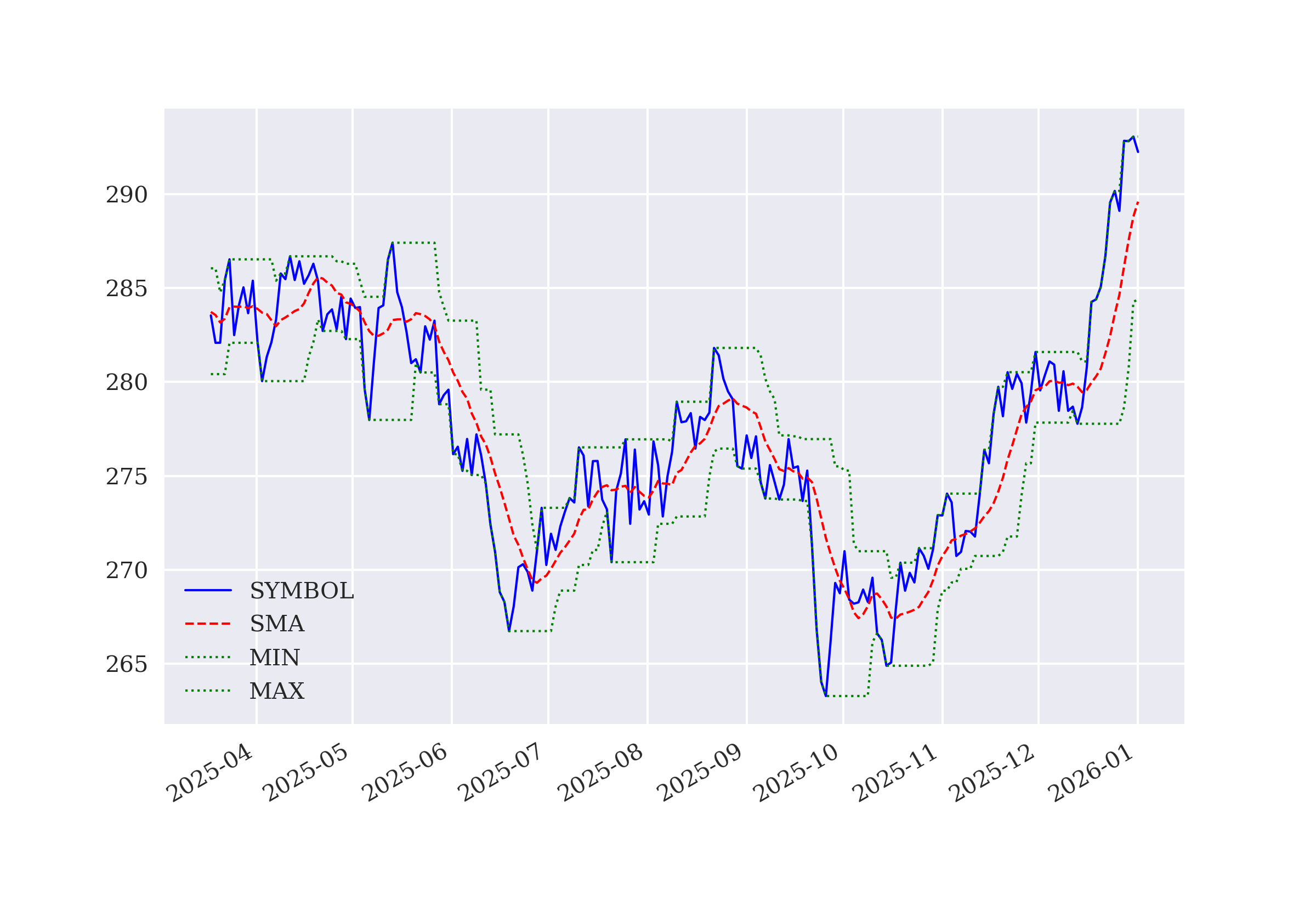
Figure 15. Simulated financial time series data with multiple features

6.3. Trading Agent

As compared to the DQLAgent class from DQLAgent Class, only the DNN model architecture needs to be changed to account for multiple features. More specifically, the input layer is adjusted to accommodate multiple features with multiple lags:

In [31]: class TradingAgent(DQLAgent):
             def _create_model(self, hu, lr):
                 self.model = Sequential()
                 self.model.add(Dense(hu, input_dim=
                     self.env.lags * self.env.n_features,
                                 activation='relu'))  (1)
                 self.model.add(Flatten())  (2)
                 self.model.add(Dense(hu, activation='relu'))
                 self.model.add(Dense(2, activation='linear'))
                 self.model.compile(loss='mse',
                     optimizer=opt(learning_rate=lr))

1	The input layer allows for multiple lags and multiple features.

This already completes the setup for algorithmic trading. To have a benchmark for the algorithmically trading agent to compare with, the following code instantiates the Trading object and generates test results without any prior training. In that case, the random weights from the DNN initialization are used to generate the trading predictions. Because the environment is configured such that the simulated price process has a long-term mean (theta) well below the initial price (x0) all simulated price processes drop significantly on average in value. The random agent realizes a negative performance for all the test runs. Histogram of the test performances (random FQL agent) shows the histogram of the performances realized. The net performance is negative throughout.

In [32]: random.seed(100)
         tf.random.set_seed(100)

In [33]: trading = Trading(symbol, ['r', 'DEL', 'MOM'], window=10, lags=8,
                     start='2024-1-1', end='2026-1-1', periods=2 * 252,
                     x0=100, kappa=2, theta=50, sigma=0.1,
                     leverage=1, min_accuracy=0.5, min_performance=0.85,
                     new=True, normalize=True)

In [34]: tradingagent = TradingAgent(trading.symbol, trading.features,
                          trading.n_features, trading, hu=24, lr=0.0001)

In [35]: %%time
         tradingagent.test(100, min_accuracy=0.0,
                    min_performance=0.0,
                    verbose=True, full=False)
         total reward= 486 | accuracy=0.447 | performance=0.662
         CPU times: user 20.8 s, sys: 2.72 s, total: 23.6 s
         Wall time: 20.3 s

In [36]: random_performances = tradingagent.performances  (1)

In [37]: sum(random_performances) / len(random_performances)  (2)
Out[37]: 0.7349392873819823

In [38]: plt.hist(random_performances, bins=50, color='b')
         plt.xlabel('gross performance')
         plt.ylabel('frequency');

1	Stores the realized performances of the random DQL agent.
2	Calculates the average gross performance of the random DQL agent.

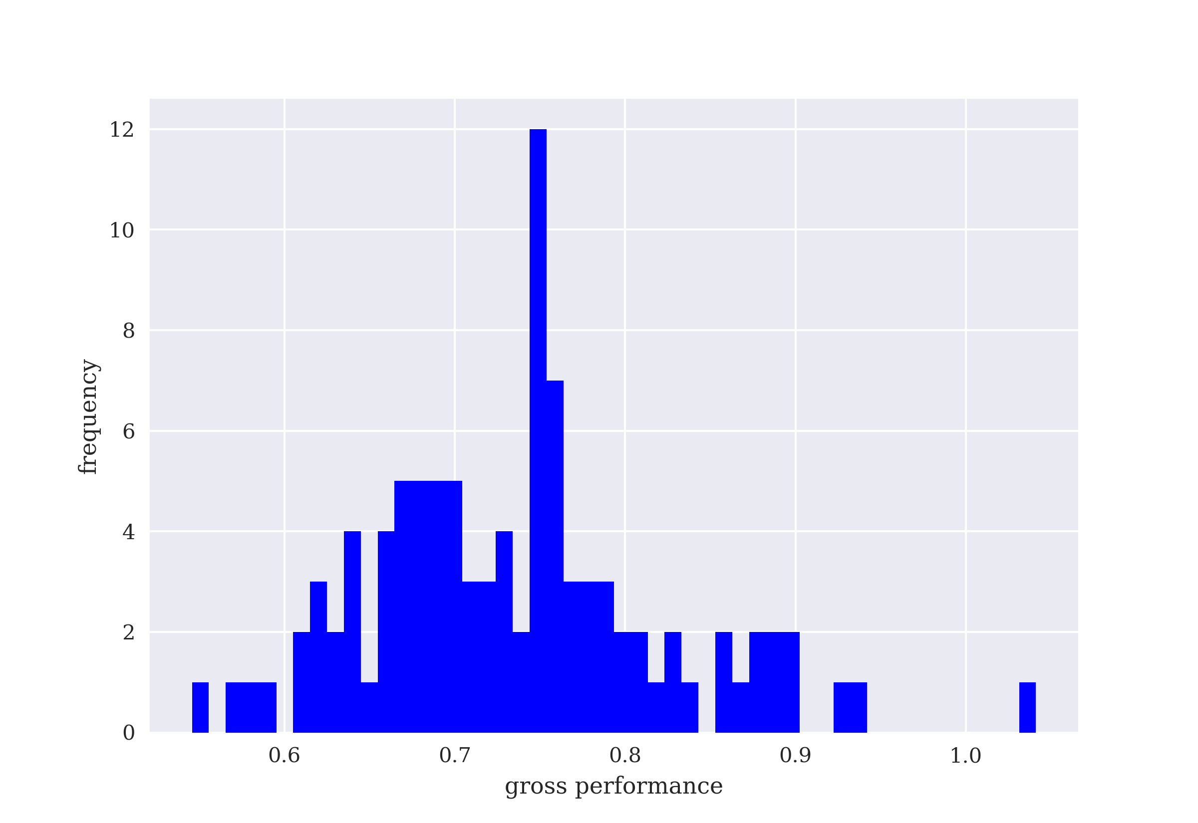
Figure 16. Histogram of the test performances (random FQL agent)

The following code trains the TradingAgent and updates the weights in the neural network accordingly. The agent learns that the simulated time series drop on average and takes on more short positions to benefit from the falling price. It generates a significantly positive average performance, illustrating the superiority of the trained agent over a simple random agent. Not a single time does the trained agent lose money. Histogram of the test performances (trained vs. random FQL agent) shows the histogram of the performances realized in comparison to those of the random agent.

In [39]: %time tradingagent.learn(500)
         episode= 500 | treward= 280.00 | max= 295.00
         CPU times: user 58.3 s, sys: 7.56 s, total: 1min 5s
         Wall time: 56.2 s

In [40]: %%time
         tradingagent.test(50, min_accuracy=0.0,
                    min_performance=0.0,
                    verbose=True, full=False)
         total reward= 486 | accuracy=0.549 | performance=1.582
         CPU times: user 10.6 s, sys: 1.34 s, total: 11.9 s
         Wall time: 10.4 s

In [41]: sum(tradingagent.performances) / len(tradingagent.performances)
Out[41]: 1.6505126231620155

In [42]: plt.hist(random_performances, bins=30,
                  color='b', label='random (left)')
         plt.hist(tradingagent.performances, bins=30,
                  color='r', label='trained(right)')
         plt.xlabel('gross performance')
         plt.ylabel('frequency')
         plt.legend();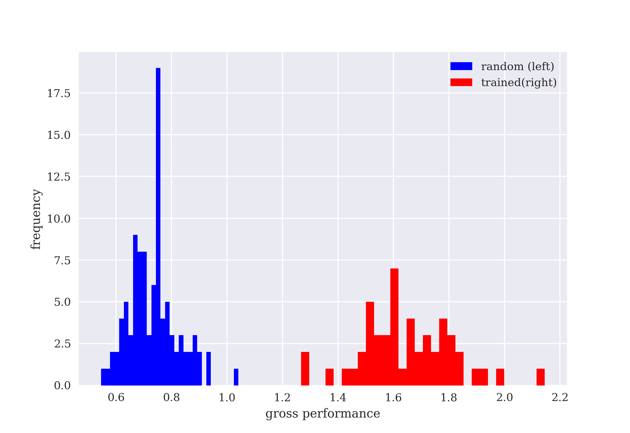

Figure 17. Histogram of the test performances (trained vs. random FQL agent)

6.4. Conclusions

This chapter discusses deep Q-learning for algorithmic trading. The setup is close to the financial prediction game as discussed in Financial Q-Learning which is why it is presented as the first financial application in Financial Applications.

The chapter uses a TradingAgent class that inherits from the DQLAgent class of DQLAgent Class and that allows not only for consistency with the previous environments introduced in the book but also for a richer state space with multiple features and multiple lags. The only adjustment necessary to accommodate multiple features is with regard to the input layer of the neural network. The Trading environment is based on a Monte Carlo simulation approach as introduced in Simulated Time Series Data and adds multiple financial features that the TradingAgent can choose from.

Trading Agent shows that the TradingAgent can easily learn that the simulated price processes drop over time and outperforms a random agent by a large margin.

Hilpisch (2020) provides more details about DQL in the context of algorithmic trading. Among other things, the book shows how to backtest the performance of a DQL agent with vectorized and event-based backtesting. It also shows how to deploy a trained DQL agent for live algorithmic trading via API access to a trading platform.

The next chapter turns attention to the application of DQL to the problem of learning how to dynamically hedge (or delta hedge) a European call option.

6.5. References

Books and articles cited in this chapter:

Bostrom, Nick (2014): Superintelligence: Paths, Dangers, Strategies. Oxford University Press, Oxford.
Hilpisch, Yves (2020): Artificial Intelligence in Finance—A Python-Based Guide. O’Reilly, Sebastopol.
Maney, Kevin (2017): “Goldman Sacked: How AI Will Transform Wall Street.” Newsweek, 10. March 2017.
Vasicek, Oldrich (1977): “An equilibrium characterization of the term structure.” Journal of Financial Economics, Vol. 5, No. 2, 177–188.

6.6. Finance Environment

The Python module finance.py provides the Finance class from Financial Q-Learning:

#
# Finance Environment with Historical Data
#
# (c) Dr. Yves J. Hilpisch
# Reinforcement Learning for Finance
#

import random
import numpy as np
import pandas as pd


class ActionSpace:
    def sample(self):
        return random.randint(0, 1)


class Finance:
    url = 'https://certificate.tpq.io/rl4finance.csv'
    def __init__(self, symbol, feature, min_accuracy=0.485, n_features=4):
        self.symbol = symbol
        self.feature = feature
        self.n_features = n_features
        self.action_space = ActionSpace()
        self.min_accuracy = min_accuracy
        self._get_data()
        self._prepare_data()

    def _get_data(self):
        self.raw = pd.read_csv(self.url,
                index_col=0, parse_dates=True)

    def _prepare_data(self):
        self.data = pd.DataFrame(self.raw[self.symbol]).dropna()
        self.data['r'] = np.log(self.data / self.data.shift(1))
        self.data['d'] = np.where(self.data['r'] > 0, 1, 0)
        self.data.dropna(inplace=True)
        self.data_ = (self.data - self.data.mean()) / self.data.std()

    def reset(self):
        self.bar = self.n_features
        self.treward = 0
        state = self.data_[self.feature].iloc[
            self.bar - self.n_features:self.bar].values
        return state, {}
        
    def step(self, action):
        if action == self.data['d'].iloc[self.bar]:
            correct = True
        else:
            correct = False
        reward = 1 if correct else 0
        self.treward += reward
        self.bar += 1
        self.accuracy = self.treward / (self.bar - self.n_features)
        if self.bar >= len(self.data):
            done = True
        elif reward == 1:
            done = False
        elif (self.accuracy < self.min_accuracy) and (self.bar > 15):
            done = True
        else:
            done = False
        next_state = self.data_[self.feature].iloc[
            self.bar - self.n_features:self.bar].values
        return next_state, reward, done, False, {}

6.7. DQLAgent Class

The Python module dqlagent.py provides the DQLAgent class from Financial Q-Learning. The version presented here implements several adjustments and generalizations to allow, among other things, for multiple features instead of just one. Other changes are minor and generally technical in nature.

#
# Deep Q-Learning Agent
#
# (c) Dr. Yves J. Hilpisch
# Reinforcement Learning for Finance
#

import os
import random
import warnings
import numpy as np
import tensorflow as tf
from tensorflow import keras
from collections import deque
from keras.layers import Dense, Flatten
from keras.models import Sequential

warnings.simplefilter('ignore')
os.environ['TF_CPP_MIN_LOG_LEVEL'] = '3'


from tensorflow.python.framework.ops import disable_eager_execution
disable_eager_execution()

opt = keras.optimizers.legacy.Adam


class DQLAgent:
    def __init__(self, symbol, feature, n_features, env, hu=24, lr=0.001):
        self.epsilon = 1.0
        self.epsilon_decay = 0.9975
        self.epsilon_min = 0.1
        self.memory = deque(maxlen=2000)
        self.batch_size = 32
        self.gamma = 0.5
        self.trewards = list()
        self.max_treward = -np.inf
        self.n_features = n_features
        self.env = env
        self.episodes = 0
        self._create_model(hu, lr)
        
    def _create_model(self, hu, lr):
        self.model = Sequential()
        self.model.add(Dense(hu, activation='relu',
                             input_dim=self.n_features))
        self.model.add(Dense(hu, activation='relu'))
        self.model.add(Dense(2, activation='linear'))
        self.model.compile(loss='mse', optimizer=opt(learning_rate=lr))
        
    def _reshape(self, state):
        state = state.flatten()
        return np.reshape(state, [1, len(state)])
            
    def act(self, state):
        if random.random() < self.epsilon:
            return self.env.action_space.sample()
        return np.argmax(self.model.predict(state)[0])
        
    def replay(self):
        batch = random.sample(self.memory, self.batch_size)
        for state, action, next_state, reward, done in batch:
            if not done:
                reward += self.gamma * np.amax(
                    self.model.predict(next_state)[0])
                target = self.model.predict(state)
                target[0, action] = reward
                self.model.fit(state, target, epochs=1, verbose=False)
        if self.epsilon > self.epsilon_min:
            self.epsilon *= self.epsilon_decay
            
    def learn(self, episodes):
        for e in range(1, episodes + 1):
            self.episodes += 1
            state, _ = self.env.reset()
            state = self._reshape(state)
            treward = 0
            for f in range(1, 5000):
                self.f = f
                action = self.act(state)
                next_state, reward, done, trunc, _ = self.env.step(action)
                treward += reward
                next_state = self._reshape(next_state)
                self.memory.append(
                    [state, action, next_state, reward, done])
                state = next_state 
                if done:
                    self.trewards.append(treward)
                    self.max_treward = max(self.max_treward, treward)
                    templ = f'episode={self.episodes:4d} | '
                    templ += f'treward={treward:7.3f}'
                    templ += f' | max={self.max_treward:7.3f}'
                    print(templ, end='\r')
                    break
            if len(self.memory) > self.batch_size:
                self.replay()
        print()
        
    def test(self, episodes, min_accuracy=0.0,
             min_performance=0.0, verbose=True,
             full=True):
        ma = self.env.min_accuracy
        self.env.min_accuracy = min_accuracy
        if hasattr(self.env, 'min_performance'):
            mp = self.env.min_performance
            self.env.min_performance = min_performance
            self.performances = list()
        for e in range(1, episodes + 1):
            state, _ = self.env.reset()
            state = self._reshape(state)
            for f in range(1, 5001):
                action = np.argmax(self.model.predict(state)[0])
                state, reward, done, trunc, _ = self.env.step(action)
                state = self._reshape(state)
                if done:
                    templ = f'total reward={f:4d} | '
                    templ += f'accuracy={self.env.accuracy:.3f}'
                    if hasattr(self.env, 'min_performance'):
                        self.performances.append(self.env.performance)
                        templ += f' | performance={self.env.performance:.3f}'
                    if verbose:
                        if full:
                            print(templ)
                        else:
                            print(templ, end='\r')
                    break
        self.env.min_accuracy = ma
        if hasattr(self.env, 'min_performance'):
            self.env.min_performance = mp
        print()

6.8. Simulation Environment

The Python module simulation.py provides the Simulation class from Simulated Time Series Data:

#
# Monte Carlo Simulation Environment
#
# (c) Dr. Yves J. Hilpisch
# Reinforcement Learning for Finance
#

import math
import random
import numpy as np
import pandas as pd
from numpy.random import default_rng

rng = default_rng()


class ActionSpace:
    def sample(self):
        return random.randint(0, 1)


class Simulation:
    def __init__(self, symbol, feature, n_features,
                 start, end, periods,
                 min_accuracy=0.525, x0=100,
                 kappa=1, theta=100, sigma=0.2,
                 normalize=True, new=False):
        self.symbol = symbol
        self.feature = feature
        self.n_features = n_features
        self.start = start
        self.end = end
        self.periods = periods
        self.x0 = x0
        self.kappa = kappa
        self.theta = theta
        self.sigma = sigma
        self.min_accuracy = min_accuracy
        self.normalize = normalize
        self.new = new
        self.action_space = ActionSpace()
        self._simulate_data()
        self._prepare_data()

    def _simulate_data(self):
        index = pd.date_range(start=self.start,
                    end=self.end, periods=self.periods)
        s = [self.x0]
        dt = (index[-1] - index[0]).days / 365 / self.periods
        for t in range(1, len(index)):
            s_ = (s[t - 1] + self.kappa * (self.theta - s[t - 1]) * dt +
                  s[t - 1] * self.sigma * math.sqrt(dt) * random.gauss(0, 1))
            s.append(s_)
        
        self.data = pd.DataFrame(s, columns=[self.symbol], index=index)

    def _prepare_data(self):
        self.data['r'] = np.log(self.data / self.data.shift(1))
        self.data.dropna(inplace=True)
        if self.normalize:
            self.mu = self.data.mean()
            self.std = self.data.std()
            self.data_ = (self.data - self.mu) / self.std
        else:
            self.data_ = self.data.copy()
        self.data['d'] = np.where(self.data['r'] > 0, 1, 0)
        self.data['d'] = self.data['d'].astype(int)

    def _get_state(self):
        return self.data_[self.feature].iloc[self.bar -
                                self.n_features:self.bar]
        
    def seed(self, seed):
        random.seed(seed)
        np.random.seed(seed)
        tf.random.set_random_seed(seed)
        
    def reset(self):
        if self.new:
            self._simulate_data()
            self._prepare_data()
        self.treward = 0
        self.accuracy = 0
        self.bar = self.n_features
        state = self._get_state()
        return state.values, {}

    def step(self, action):
        if action == self.data['d'].iloc[self.bar]:
            correct = True
        else:
            correct = False
        reward = 1 if correct else 0 
        self.treward += reward
        self.bar += 1
        self.accuracy = self.treward / (self.bar - self.n_features)
        if self.bar >= len(self.data):
            done = True
        elif reward == 1:
            done = False
        elif (self.accuracy < self.min_accuracy and
              self.bar > self.n_features + 15):
            done = True
        else:
            done = False
        next_state = self.data_[self.feature].iloc[
            self.bar - self.n_features:self.bar].values
        return next_state, reward, done, False, {}

7. Dynamic Hedging

Before the advent of Black-Scholes, option markets were sparse and thinly traded. Now they are among the largest and most active security markets. The change is attributed by many to the Black-Scholes model, since it provides a benchmark for valuation and (via the arbitrage argument) a method for replicating or hedging options positions.

— Duffie (1998)

Algorithmic Trading uses DQL to learn “how to beat the markets”, that is, to learn to enter long and short positions in a financial instrument in a way that outperforms a benchmark strategy such as, for example, simply going long the financial instrument. This can be interpreted as trying to prove the efficient market hypothesis (EMH) wrong. Simply speaking, the so-called weak-form EMH postulates that market-observed prices reflect all publicly available information. Timmermann and Granger (2004) provide a modern perspective on and definition of the EMH.

In option pricing, or more generally derivative pricing, one generally takes the viewpoint that the market is always right and that one can leverage what is observed in the markets to price derivative instruments whose prices might not be directly observable. In other words, one trusts that markets are efficient and that the EMH holds. This in turn builds the basis for strong arbitrage pricing arguments: two financial instruments have to have the same price if they generate the exact same payoffs in the future. A portfolio of, say, a stock and a bond position that pays off the same in the future as a European call option on the stock — so the argument goes — therefore must have the same market price.

Mathematical finance researchers have proposed several different models that leverage the EMH and arbitrage arguments to derive values for derivative instruments. This chapter focuses on the seminal works by Black and Scholes (1973) and Merton (1973), together for short BSM73. In this context, refer also the survey paper by Duffie (1998).

Delta Hedging introduces the major elements of the model, discusses delta hedging and option replication, and illustrates numerically how option replication can be accomplished through dynamically trading a risky and a risk-less asset, say, a stock and a bond. In this context, dynamic hedging, delta hedging, dynamic replication, and option replication are used interchangeably although there might be differences in practice concerning their goals and implementations. The book by Taleb (1996) provides an in-depth treatment of the theoretical and practical aspects of dynamic hedging. Hedging Environment develops a financial environment that is suited to simulate the dynamic replication of an option. Hedging Agent adjusts the DQL agent from DQLAgent Class in a way that the resulting HedgingAgent class can learn option replication in the model of BSM73. The agent learns the dynamic replication of a European call option just by observing a subset of the model parameters and the option price. As is usual throughout the book, the agent does not have any knowledge of the model itself (“model-free” learning), the delta, or how delta can be derived and used.

7.1. Delta Hedging

This section discusses the seminal option pricing model by BSM73 and how to implement delta hedging. The BSM73 model is based on geometric Brownian motion (GBM) which is a special case of the Vasicek (1977) Ornstein-Uhlenbeck process introduced in Simulated Time Series Data. GBM is a process to describe the evolution of stochastic quantities in continuous time. The resulting prices are log-normally distributed while the resulting returns are normally distributed.

The BSM73 model assumes that there are two traded assets, a risky one and a risk-less one. In BSM73, the GBM describes the stochastic evolution of the risky asset, such as a stock or an equity index. The stochastic differential equation (SDE) for the GBM is as follows:

\[dS_t = \mu S_t dt + \sigma S_t dZ_t\]

The variables have the following meanings: $S_t$ is the index level at time $t$, $\mu$ is the constant drift factor, $\sigma$ is the constant volatility (= standard deviation of returns) of $S$, and $Z_t$ is a standard, arithmetic Brownian motion (or Wiener process).

In general, a fixed initial value for $S_0$ is assumed as an initial boundary condition. In a risk-neutral pricing context, the constant drift factor $\mu$ is replaced by the constant risk-less short rate $r$, leading to the following alternative SDE describing the evolution of the marginal return of the risky asset:

\[\frac{dS_t}{S_t} = r dt + \sigma dZ_t\]

This illustrates the normal distribution of the marginal returns. Given some initial value $B_0$, the returns process of the risk-less asset, such as a bond or a money market account, is deterministic:

\[\frac{dB_t}{B_t} = e^{rt}\]

In this version of the BSM73 model, no dividends are assumed such that the risky asset is generally thought of as an equity index or a similar financial instrument without any dividend payments.^[22]

Now consider a European call option on the risky asset with fixed strike price $K$ and a fixed maturity date $T$. The payoff $h_t$ of the option at maturity is given by

\[h_T = \max(S_T - K, 0)\]

On the one hand, such an option gives the right to buy the risky asset at the strike price at maturity. This is advantageous whenever $S_T > K$ holds at maturity. On the other hand, there is no obligation for the option holder to do so. In other words, the option holder only realizes a positive payoff at maturity or one of zero as the fixed minimum — that is, the option expires worthless. It can be shown that the arbitrage-free value at time $t$ of the option is given by the following analytical formula:

\[C_t^{BSM73}(S_t, K, T, t, r, \sigma) = S_t \mathbf{N}(d_1) - e^{-r(T - t)} K \mathbf{N}(d_2)\]

where

\[\begin{array}{} \mathbf{N}(d) &=& \frac{1}{\sqrt{2 \pi}} \int_{-\infty}^{d} e^{-\frac{1}{2}x^2} dx\\ d_1 &=& \frac{\log \frac{S_t}{K} + \left( r + \frac{\sigma^2}{2} \right) (T - t)} {\sigma \sqrt{T - t}} \\ d_2 &=& \frac{\log \frac{S_t}{K} + \left( r - \frac{\sigma^2}{2} \right) (T - t)} {\sigma \sqrt{T - t}} \end{array}\]

The book by Baxter and Rennie (1996) provides more details about the BSM73 model and about how to derive the pricing formula through arbitrage reasoning. It also explains the methods from stochastic calculus that are needed in continuous-time pricing models. The book by Hilpisch (2015) additionally provides details about numerical methods related to this and similar option pricing models, such as Monte Carlo simulation, and their implementation in Python.

BSM (1973) Formula shows the Python module that implements the BSM73 pricing formula for European call options. Its application is straightforward once the model parameters are fixed. To get started, the usual imports first:

In [58]: import math
         import random
         import numpy as np
         import pandas as pd
         from scipy import stats
         from pylab import plt, mpl

In [59]: plt.style.use('seaborn-v0_8')
         mpl.rcParams['figure.dpi'] = 300
         mpl.rcParams['savefig.dpi'] = 300
         mpl.rcParams['font.family'] = 'serif'
         np.set_printoptions(suppress=True)

Second, the import and application of the bsm_call_value() valuation function for BSM73:

In [60]: from bsm73 import bsm_call_value

In [61]: S0 = 100  (1)
         K = 100  (2)
         T = 1.  (3)
         t = 0.  (4)
         r = 0.05  (5)
         sigma = 0.2  (6)

In [62]: bsm_call_value(S0, K, T, t, r, sigma)
Out[62]: 10.450583572185565

1	Initial stock price.
2	Strike price of the option.
3	Maturity date in year fractions.
4	Current date in year fractions.
5	Constant risk-less short rate.
6	Constant volatility factor.

Simply speaking, there are two arguments to derive the arbitrage-free value of a European call option as embodied by the BSM73 formula:

Dynamic hedging: You can hedge the price risk of the European option by continuously trading in the underlying financial instrument in a way that the overall risk becomes zero. In equilibrium, the portfolio of the option and the hedge position must yield the risk-free rate because it is risk-free by construction.
Option replication: You can set up a replication portfolio consisting of positions in the risky and the risk-less asset. This portfolio is continuously re-balanced in a way that its value equals the value of the European option at any point in time. By arbitrage reasoning, the value of the option and the value of the replication portfolio at any time must be equal.

These two arguments represent two sides of the same coin. At their core, they both make use of the so-called delta of the option. The delta of an option measures the changes in the option’s value for a marginal price change in the risky asset from which the option derives its value. Formally, the delta or $\Delta$ of an option is defined as the first partial derivative of the option valuation formula with regard to the price of the underlying asset:

\[\Delta \equiv \frac{\partial C}{\partial S}\]

For the BSM73 model, with given parameters $K, T, r, \sigma$, one gets:

\[\Delta_t^{BSM73} \equiv \frac{\partial C_t^{BSM73}}{\partial S_t} = \mathbf{N}(d_1)\]

This derivation holds true for a European call option written on a single unit of the financial instrument. By construction, investing $\Delta_t^{BSM73} \cdot S_t$ in the underlying instrument shows the same profit or loss (P&L) over very short periods. Analogously, going short such a position, that is $- \Delta_t^{BSM73} \cdot S_t$, the change in the option value is offset by the hedge position over short periods.

Continuous vs. Discrete Time

Delta hedging and option replication as described in this section are based on a financial model in continuous time. This implies that traders are assumed to be able to trade basically at every instant of the relevant time interval. As a consequence, theoretical delta hedging and dynamic replication of an option will lead to infinitely many trades. This is only possible in theory because technology constraint prohibits trading at the speed of light. In a similar vein, non-zero transaction costs would lead to infinite hedging and replication costs rendering continuous trading impossible too. Taleb (1996) summarizes: “Perhaps the largest misconception in the financial markets attends the definition and meaning of the delta. Every operator instinctively knows that hedging in continuous time will never be possible.” Therefore, in practical applications delta hedging and dynamic option replication need to be implemented at discrete points in time. The time delta between such two points should not, however, be too large because hedge and replication errors would increase as a consequence.

Against this background, a replication portfolio $\phi_t$ for a given European call option at a certain point in time $t$ is given by:

\[\phi_t = s S_t + b B_t\]

with

\[\begin{array}{} s &=& \Delta_t^{BSM73} \\ b &=& C_t^{BSM73} - s S_t \end{array}\]

This approach can easily be illustrated in discrete time based on the Monte Carlo simulation of the GBM. An exact discretization for the GBM, that is, one that converges to the corresponding continuous-time process for ever smaller time intervals, is given by the so-called Euler discretization scheme. Assuming that $t$ is taken from a discrete set of equidistant points in time, $t \in \{0, \Delta, 2\Delta, \dots, T\}$, the following difference equations for the continuous market model ensue:

\[\begin{array}{} \frac{\Delta S_t}{S_t} &=& \exp\left(\left(r-\frac{\sigma^2}{2}\right) \Delta t + \sigma \sqrt{\Delta t} z_t\right) \\ \frac{\Delta B_t}{B_t} &=& e^{r \Delta t} \end{array}\]

Here, $\Delta t$ is the fixed distance between two points in time, $\Delta X_t = X_t - X_{t - \Delta t}$ is the absolute change in the price of asset $X$, and $z_t$ is a standard normally distributed random variable.

The following Python function implements Monte Carlo simulation for the GBM. Simulated price process for BSM73 model shows a resulting process.

In [63]: random.seed(1000)

In [64]: def simulate_gbm(S0, T, r, sigma, steps=100):
             gbm = [S0]
             dt = T / steps
             for t in range(1, steps + 1):
                 st = gbm[-1] * math.exp((r - sigma ** 2 / 2) * dt
                             + sigma * math.sqrt(dt) * random.gauss(0, 1))
                 gbm.append(st)
             return gbm

In [65]: gbm = simulate_gbm(S0, T, r, sigma)

In [66]: plt.plot(gbm, lw=1.0, c='b')
         plt.xlabel('time step')
         plt.ylabel('stock price');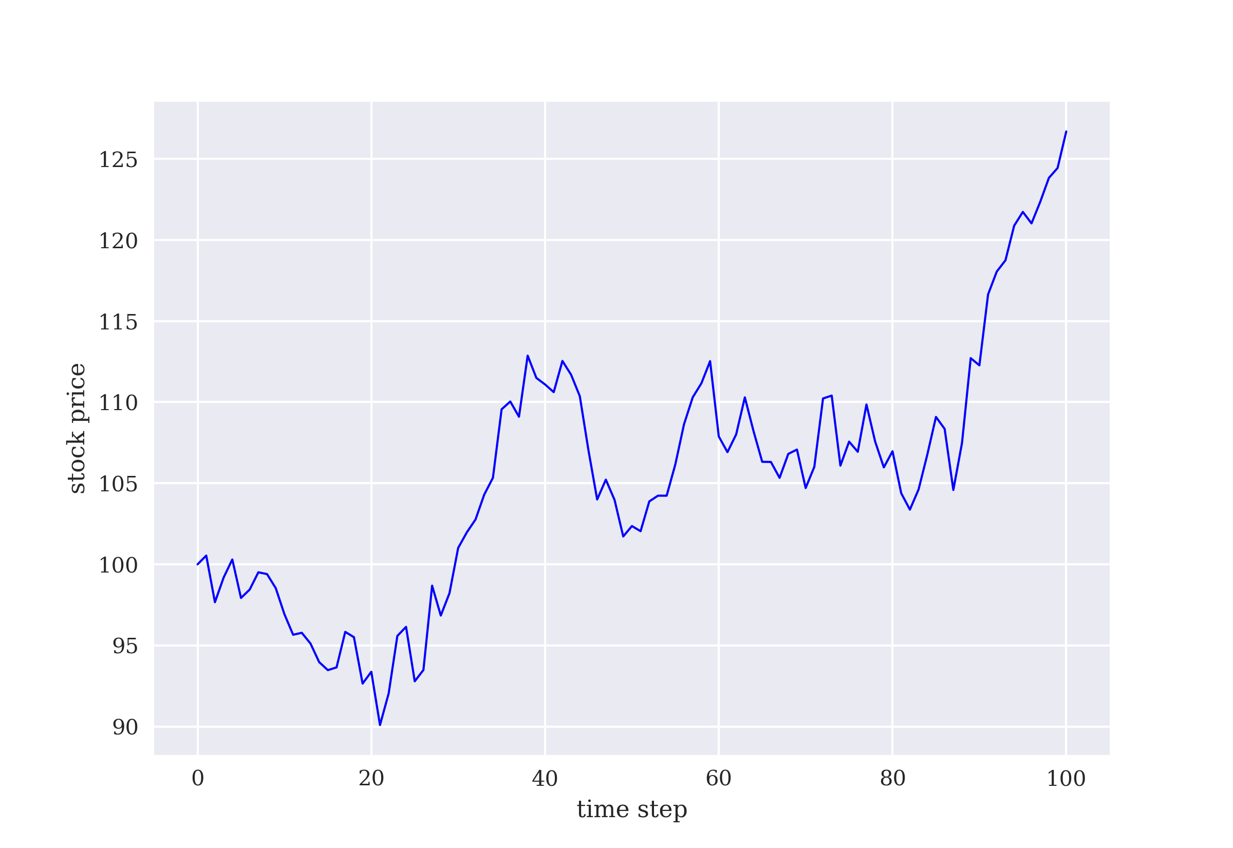

Figure 18. Simulated price process for BSM73 model

It is noteworthy that the $\Delta^{BSM73}$ of a European call option on a single unit of the underlying financial instrument only takes on values between 0 and 1. Delta for European call option in BSM73 model shows this for a larger number of different prices of the underlying.

In [67]: def bsm_delta(St, K, T, t, r, sigma):
             d1 = ((math.log(St / K) + (r + 0.5 * sigma ** 2) * (T - t)) /
                   (sigma * math.sqrt(T - t)))
             return stats.norm.cdf(d1, 0, 1)

In [68]: S_ = range(40, 181, 4)

In [69]: d = [bsm_delta(s, K, T, 0, r, sigma) for s in S_]

In [70]: plt.plot(S_, d, lw=1.0, c='b')
         plt.xlabel('stock price')
         plt.ylabel('delta');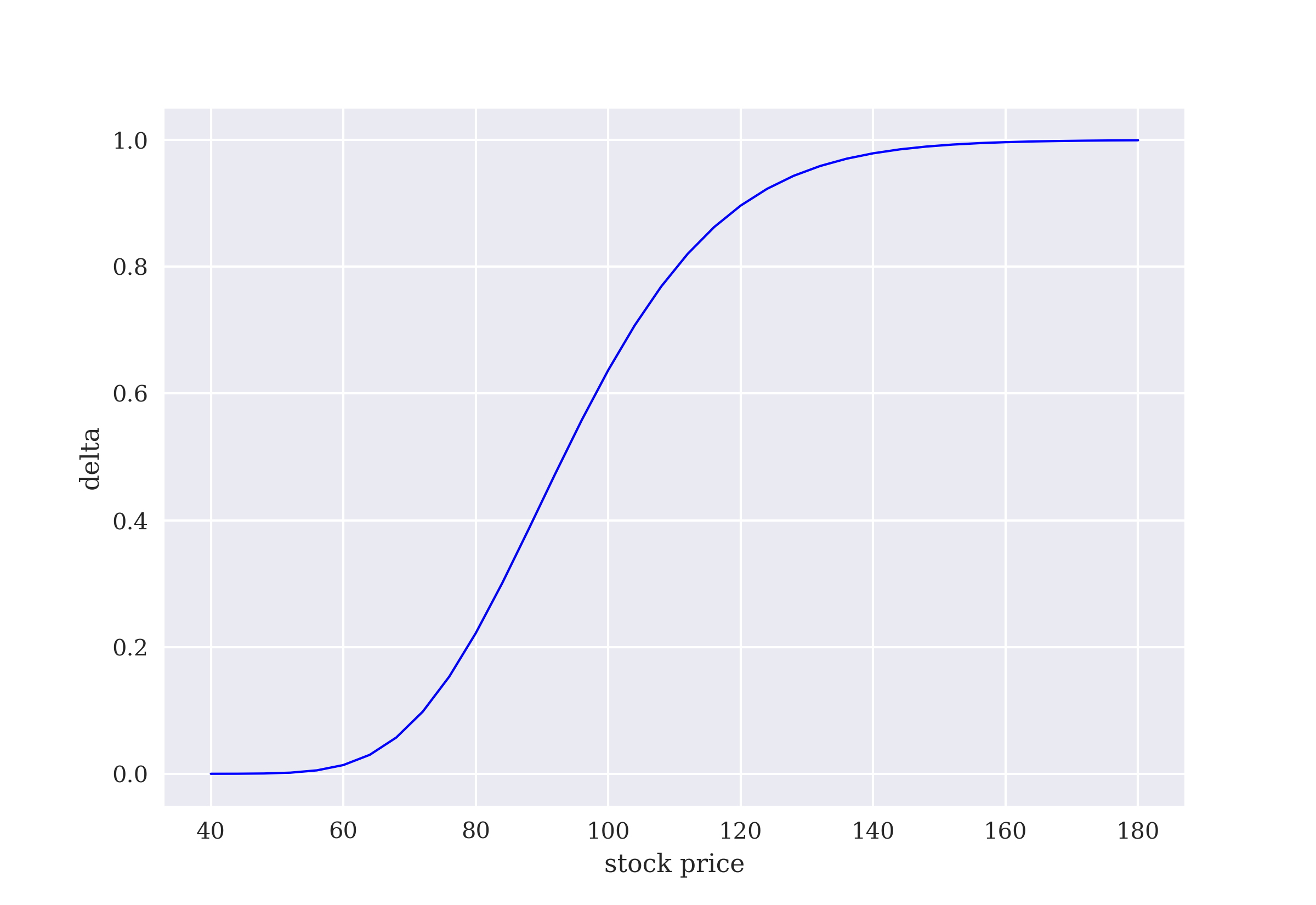

Figure 19. Delta for European call option in BSM73 model

Equipped with the function for $\Delta_t^{BSM73}$, portfolio replication in the BSM73 model can be simulated in discrete time as follows. Option value and replication portfolio value over time shows the option values and replication portfolio values over time. The replication seems to be almost perfect:

In [71]: dt = T / (len(gbm) - 1)

In [72]: bond = [math.exp(r * i * dt) for i in range(len(gbm))]

In [73]: def option_replication():
             res = pd.DataFrame()
             for i in range(len(gbm) - 1):
                 C = bsm_call_value(gbm[i], K, T, i * dt, r, sigma)
                 if i == 0:
                     s = bsm_delta(gbm[i], K, T, i * dt, r, sigma)  (1)
                     b = (C - s * gbm[i]) / bond[i]  (2)
                 else:
                     V = s * gbm[i] + b * bond[i]  (3)
                     s = bsm_delta(gbm[i], K, T, i * dt, r, sigma)  (4)
                     b = (C - s * gbm[i]) / bond[i]  (5)
                     df = pd.DataFrame({'St': gbm[i], 'C': C, 'V': V,
                                        's': s, 'b': b}, index=[0])  (6)
                     res = pd.concat((res, df), ignore_index=True)  (6)
             return res

In [74]: res = option_replication()

In [75]: res[['C', 'V']].plot(style=['b', 'r--'], lw=1)
         plt.xlabel('time step')
         plt.ylabel('value');

1	Derives the initial position in the risky asset.
2	Does the same for the risk-less asset.
3	Calculates the payoff given the previously set up replication portfolio.
4	Updates the position of the risky asset.
5	Does the same for the risk-less asset.
6	Collects all relevant parameters and values in a `DataFrame` object.

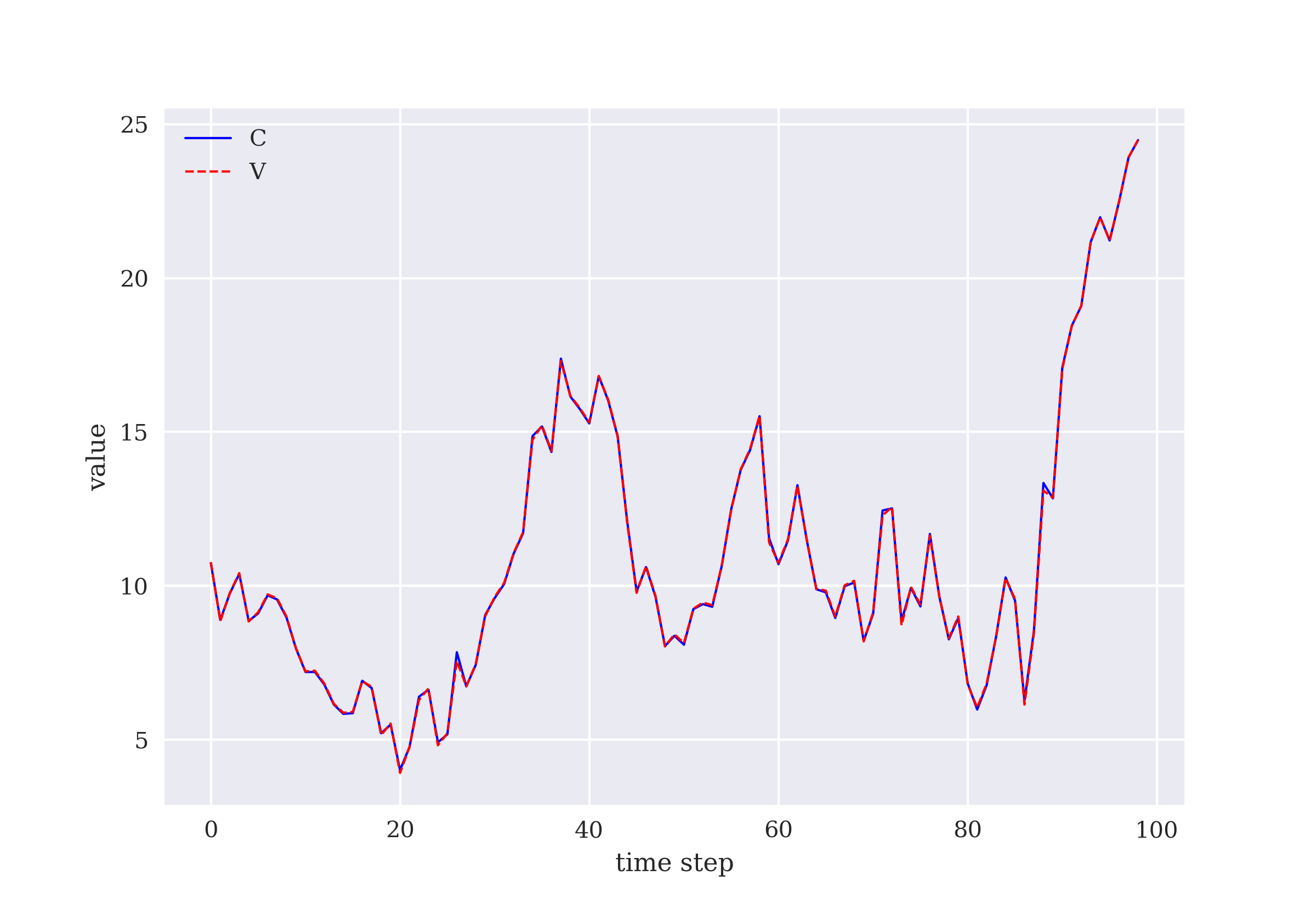
Figure 20. Option value and replication portfolio value over time

To gain more insights into how good the replication is, Replication errors for the European call option shows the profit and loss values of the replication process. The mean absolute and the mean squared errors are also calculated. They confirm that the discrete-time replication approach works quite well. The major parameter influencing the replication accuracy is the number of steps used for the discretization. The higher this number, that is, the more fine-grained the discretization, the better the results in general. They also depend on the volatility assumed, but this parameter is kept constant throughout.

In [76]: (res['V'] - res['C']).mean()  (1)
Out[76]: -0.0009828178536543022

In [77]: ((res['V'] - res['C']) ** 2).mean()  (2)
Out[77]: 0.003755015460265298

In [78]: (res['V'] - res['C']).hist(bins=35, color='b')
         plt.xlabel('P&L')
         plt.ylabel('frequency');

1	Calculates the average error.
2	Calculates the mean squared error (MSE).

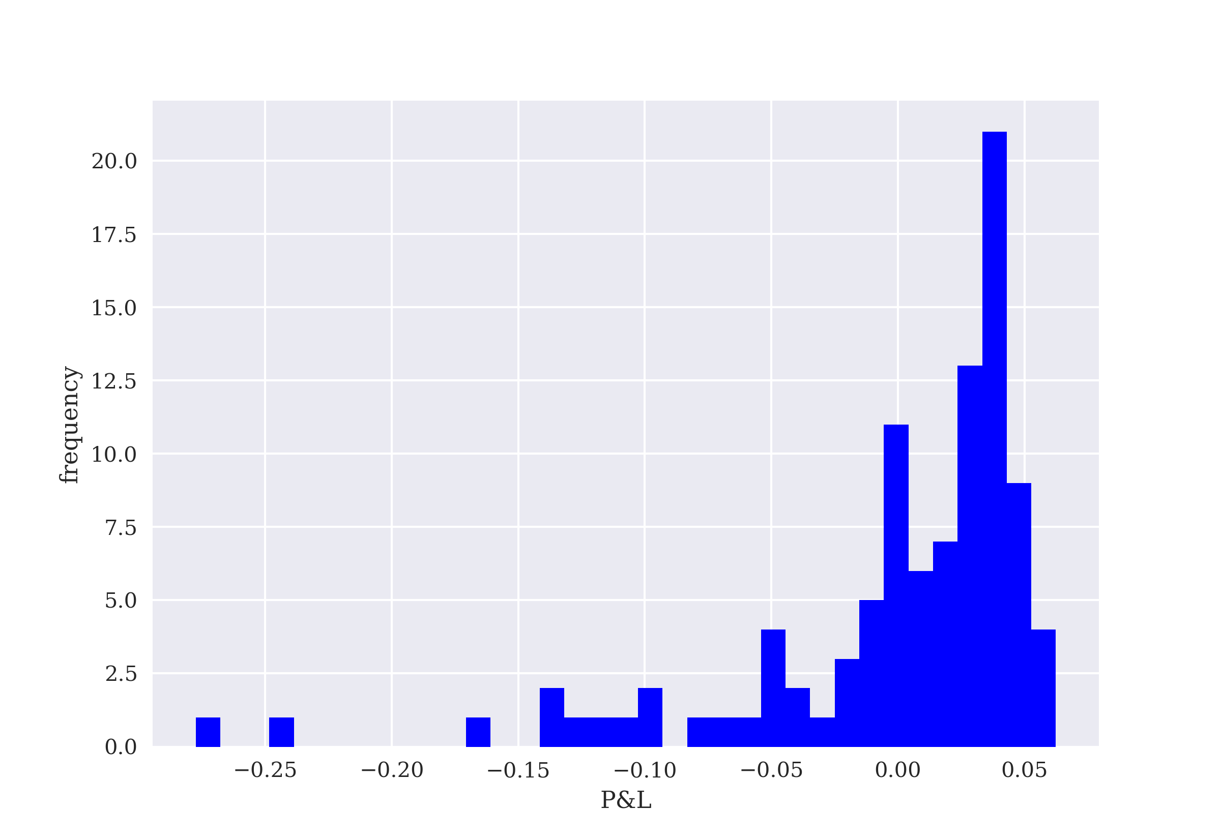
Figure 21. Replication errors for the European call option

Replication in Discrete Time

In a sandbox environment of financial markets such as the BSM73 model, dynamic replication of the European call option works quite well even in discrete time. It is quite easy to reduce the average hedge errors by making the discretization of the relevant time interval finer. In practice, additional risk factors would arise, such as changes in volatility which is assumed to be constant in the BSM73 model. There are also limits as to how often one can re-balance a portfolio given that every transaction leads to non-zero transaction costs.

7.2. Hedging Environment

The whole approach of delta hedging — or rather dynamic option replication using the delta of an option --, as presented in Delta Hedging, rests on knowing and leveraging the details of the BSM73 model with its resulting analytical formulas for the European call option value and the delta. The idea of applying DQL in this context is to learn optimal replication strategies only based on observable market parameters and feedback, that is penalties, from replication errors.

This section develops a hedging environment that is appropriate for the task. The first major difference is that the action space changes from a discrete one to a continuous one. The agent is supposed to choose a position in the underlying financial instrument of the European call option to be hedged that is between 0 and 1 and that can take on any value in between. This, for example, is already reflected in the .sample() method of the action_space class:

In [79]: class observation_space:
             def __init__(self, n):
                 self.shape = (n,)

In [80]: class action_space:
             def __init__(self, n):
                 self.n = n
             def seed(self, seed):
                 random.seed(seed)
             def sample(self):
                 return random.random()  (1)

1	Samples a random floating point number from the unit interval.

The Hedging class, which represents the environment with which the agent interacts, takes as input primarily the parameters of the BSM73 model:

In [81]: class Hedging:
             def __init__(self, S0, K_, T, r_, sigma_, steps):
                 self.initial_value = S0
                 self.strike_ = K_  (1)
                 self.maturity = T
                 self.short_rate_ = r_  (1)
                 self.volatility_ = sigma_  (1)
                 self.steps = steps
                 self.observation_space = observation_space(5)
                 self.osn = self.observation_space.shape[0]
                 self.action_space = action_space(1)
                 self._simulate_data()
                 self.portfolios = pd.DataFrame()
                 self.episode = 0

1	The parameters can be passed as iterable objects with multiple values.

The Hedging class implements the Monte Carlo simulation for the GBM based on the Euler discretization scheme. In this context, the parameter values for the strike, the short rate, and the volatility are chosen randomly:

In [82]: class Hedging(Hedging):
             def _simulate_data(self):
                 s = [self.initial_value]
                 self.strike = random.choice(self.strike_)  (1)
                 self.short_rate = random.choice(self.short_rate_)  (1)
                 self.volatility = random.choice(self.volatility_)  (1)
                 self.dt = self.maturity / self.steps
                 for t in range(1, self.steps + 1):
                     st = s[t - 1] * math.exp(
                       ((self.short_rate - 1 / 2 * self.volatility ** 2) * self.dt +
                         self.volatility * math.sqrt(self.dt) * random.gauss(0, 1))
                     )  (2)
                     s.append(st)
                 self.data = pd.DataFrame(s, columns=['index'])
                 self.data['bond'] = np.exp(self.short_rate *
                                     np.arange(len(self.data)) * self.dt)

1	Randomly selects the parameter values.
2	Implements the Euler discretization scheme.

The state of the environment is given by five different, market observable parameters:

Current price of the underlying.
Time-to-maturity for the option.
Option value according to BSM73.
Stock position chosen by the agent.
Bond position derived from the option value and stock position.

In [83]: class Hedging(Hedging):
             def _get_state(self):
                 St = self.data['index'].iloc[self.bar]
                 Bt = self.data['bond'].iloc[self.bar]
                 ttm = self.maturity - self.bar * self.dt
                 if ttm > 0:
                     Ct = bsm_call_value(St, self.strike,
                                    self.maturity, self.bar * self.dt,
                                    self.short_rate, self.volatility)
                 else:
                     Ct = max(St - self.strike, 0)
                 return np.array([St, Bt, ttm, Ct, self.strike, self.short_rate,
                                  self.stock, self.bond]), {}
             def seed(self, seed=None):
                 if seed is not None:
                     random.seed(seed)
             def reset(self):
                 self.bar = 0
                 self.bond = 0
                 self.stock = 0
                 self.treward = 0
                 self.episode += 1
                 self._simulate_data()
                 self.state, _ = self._get_state()
                 return self.state, _

The .step() method is, as before, at the core of the environment. Here, it distinguishes between the initial action and all subsequent actions. The reward is calculated based on the P&L that the replication portfolio generates for the step. All relevant data points are collected for further analysis after the training of the RL agent:

In [84]: class Hedging(Hedging):
             def step(self, action):
                 if self.bar == 0:  (1)
                     reward = 0
                     self.bar += 1
                     self.stock = float(action)  (2)
                     self.bond = ((self.state[3] - self.stock * self.state[0]) /
                                  self.state[1])  (3)
                     self.new_state, _ = self._get_state()
                 else:
                     self.bar += 1
                     self.new_state, _ = self._get_state()
                     phi_value = (self.stock * self.new_state[0] +
                            self.bond * self.new_state[1])  (4)
                     pl = phi_value - self.new_state[3]  (5)
                     df = pd.DataFrame({'e': self.episode, 's': self.stock,
                                        'b': self.bond, 'phi': phi_value,
                                        'C': self.new_state[3], 'p&l[$]': pl,
                                        'p&l[%]': pl / max(self.new_state[3], 1e-4) * 100,
                                        'St': self.new_state[0],
                                        'Bt': self.new_state[1],
                                        'K': self.strike, 'r': self.short_rate,
                                        'sigma': self.volatility}, index=[0])  (6)
                     self.portfolios = pd.concat((self.portfolios, df),
                                                 ignore_index=True)  (6)
                     reward = -(phi_value - self.new_state[3]) ** 2  (7)
                     self.stock = float(action)  (2)
                     self.bond = ((self.new_state[3] -
                                   self.stock * self.new_state[0]) /
                                   self.new_state[1])  (3)
                 if self.bar == len(self.data) - 1:  (8)
                     done = True
                 else:
                     done = False
                 self.state = self.new_state
                 return self.state, float(reward), done, False, {}

1	The initial action is treated separately.
2	Updates the stock position of the replication portfolio.
3	Calculates and updates the bond position.
4	Calculates the payoff of the replication portfolio.
5	Derives the P&L given the replication portfolio payoff and the option value.
6	Collects the data points for the environment in a `DataFrame` object.
7	Derives the reward based on the squared P&L, that is, the the squared difference between the replicating portfolio and the call option value.
8	Hedging takes place until one step before maturity.

The following Python code instantiates a Hedging environment object and shows the first simulated price processes for the risky asset (see Normalized price processes for risky and risk-less asset):

In [85]: S0 = 100.

In [86]: hedging = Hedging(S0=S0,
                       K_=np.array([0.9, 0.95, 1., 1.05, 1.10]) * S0,
                       T=1.0, r_=[0, 0.01, 0.05],
                       sigma_=[0.1, 0.15, 0.2], steps=2 * 252)

In [87]: hedging.seed(750)

In [88]: hedging._simulate_data()
         (hedging.data / hedging.data.iloc[0]).plot(
             lw=1.0, style=['r--', 'b-.'])
         plt.xlabel('time step')
         plt.ylabel('price');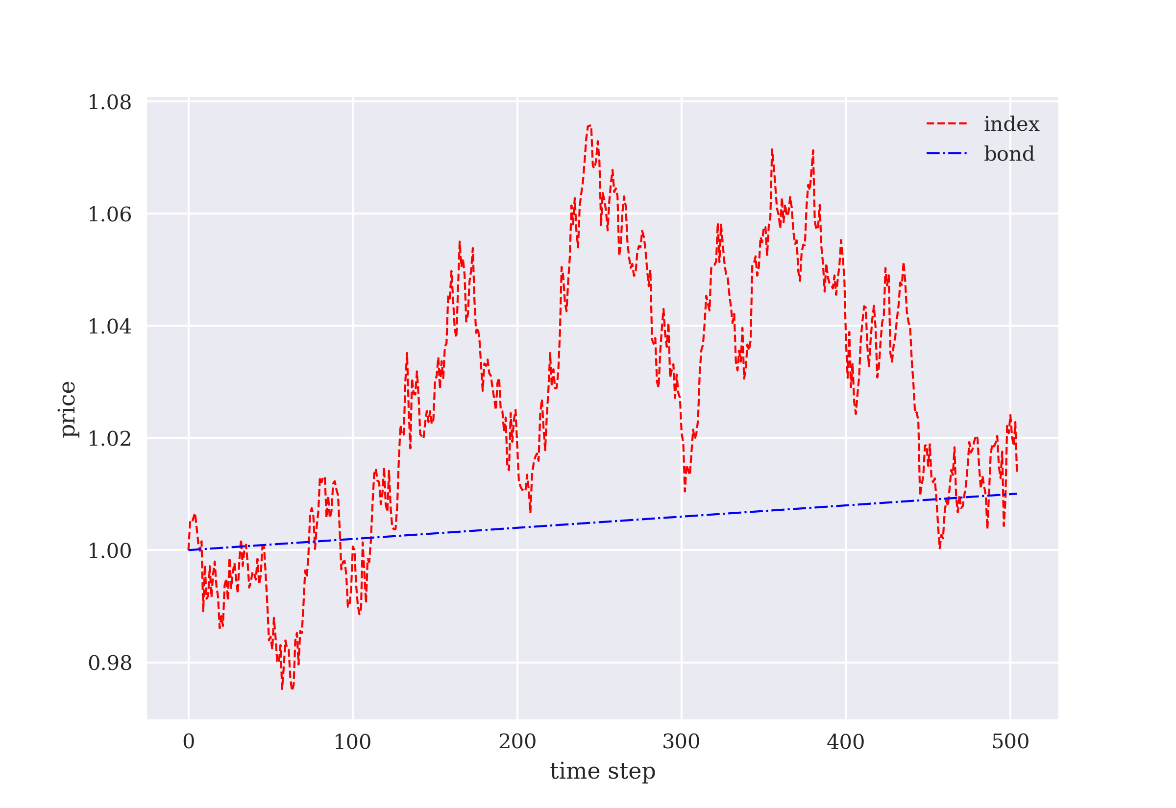

Figure 22. Normalized price processes for risky and risk-less asset

With the Hedging environment instantiated, the performance of a random hedging agent can be easily illustrated. The random hedging agent samples the stock position for the replication portfolio uniformly from the unit interval. Often, the portfolio payoff deviates significantly from the option value (see Option values (C) and random replication portfolio payoffs (phi)). Also, the portfolio payoff can take on significantly negative values which is excluded by definition for the option value:

In [89]: hedging.reset()
         for _ in range(hedging.steps - 1):
             hedging.step(hedging.action_space.sample())

In [90]: hedging.portfolios.head().round(4)
Out[90]:    e       s        b     phi       C  p&l[$]  p&l[%]        St   Bt      K  \
         0  1  0.2678 -22.4876  3.8871  3.7649  0.1222  3.2447   98.4880  1.0  110.0
         1  1  0.5623 -51.6103  4.7116  4.3306  0.3809  8.7957  100.1716  1.0  110.0
         2  1  0.5996 -55.7307  4.3350  4.3258  0.0092  0.2131  100.1789  1.0  110.0
         3  1  0.8360 -79.4251  4.7708  4.5103  0.2605  5.7760  100.7111  1.0  110.0
         4  1  0.0274   1.7478  4.5084  4.4776  0.0308  0.6877  100.6422  1.0  110.0

            r  sigma
         0  0    0.2
         1  0    0.2
         2  0    0.2
         3  0    0.2
         4  0    0.2

In [91]: hedging.portfolios[['C', 'phi']].plot(
             style=['r--', 'b-'], lw=1, alpha=0.7)
         plt.xlabel('time step')
         plt.ylabel('value');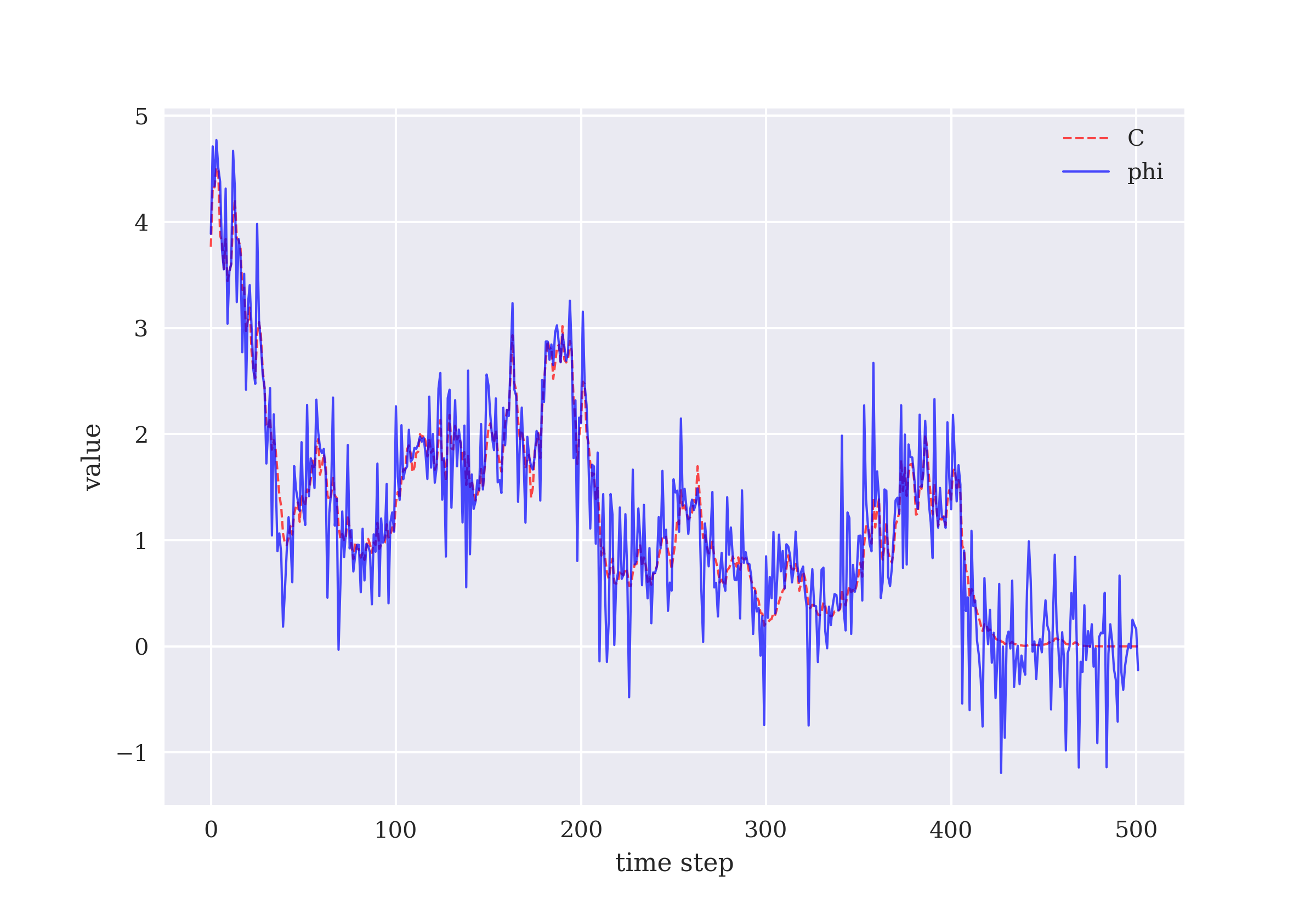

Figure 23. Option values (C) and random replication portfolio payoffs (phi)

Histogram of the P&L for the random replication strategy shows the histogram of the P&L in absolute terms for the random replication strategy.

In [92]: hedging.portfolios['p&l[$]'].apply(abs).sum()
Out[92]: 133.4348359335141

In [93]: hedging.portfolios['p&l[$]'].hist(bins=35, color='b')
         plt.xlabel('P&L')
         plt.ylabel('frequency');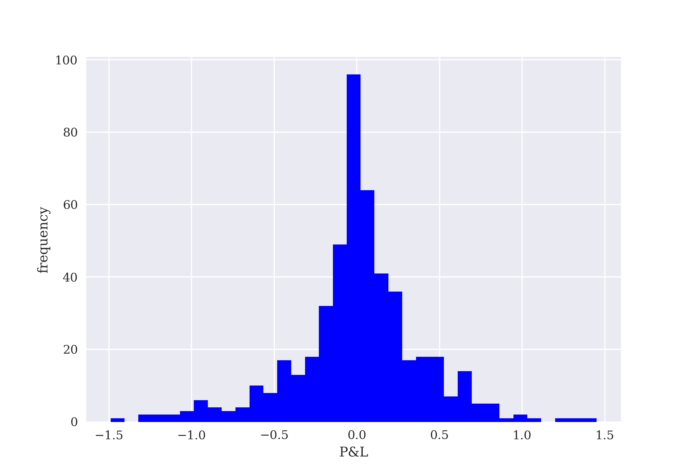

Figure 24. Histogram of the P&L for the random replication strategy

7.3. Hedging Agent

This section develops a DQL agent that learns how to dynamically replicate a European call option through interaction with the Hedging environment. Compared to the DQLAgent from DQLAgent Class, several changes need to be made. One major change is that the agent has to choose an action from an infinite number of options. This is usually called an optimal control problem. An action represents a value between 0 and 1, in line with the possible values for the delta of a European call option in the BSM73 model.

The following code inherits from the DQLAgent class from DQLAgent Class. The first major change is that the output layer now yields one floating point value only. It gives the discounted total rewards according to the DNN, given the state of the environment and a portfolio consisting of a stock and bond position:

In [94]: from dqlagent import *

In [95]: random.seed(100)
         tf.random.set_seed(100)

In [96]: opt = keras.optimizers.legacy.Adam

In [97]: class HedgingAgent(DQLAgent):
             def _create_model(self, hu, lr):
                 self.model = Sequential()
                 self.model.add(Dense(hu, input_dim=self.n_features,
                                 activation='relu'))
                 self.model.add(Dense(hu, activation='relu'))
                 self.model.add(Dense(1, activation='linear'))  (1)
                 self.model.compile(loss='mse',
                         optimizer=opt(learning_rate=lr))

1	Single valued linear output layer.

The next major change is to the selection of an optimal action. This is accomplished through an optimization procedure. Simply speaking, the agent chooses the stock position that maximizes the total reward according to the DNN:

In [98]: from scipy.optimize import minimize

In [100]: class HedgingAgent(HedgingAgent):
              def opt_action(self, state):
                  bnds = [(0, 1)]  (1)
                  def f(state, x):  (2)
                      s = state.copy()
                      s[0, 6] = x  (3)
                      s[0, 7] = ((s[0, 3] - x * s[0, 0]) / s[0, 1])  (4)
                      return self.model.predict(s)[0, 0]  (5)
                  try:
                      action = minimize(lambda x: -f(state, x), 0.5,
                                        bounds=bnds, method='Powell',
                                       )['x'][0]  (6)
                  except:
                      action = self.env.stock
                  return action

              def act(self, state):
                  if random.random() <= self.epsilon:
                      return self.env.action_space.sample()
                  action = self.opt_action(state)  (7)
                  return action

1	The bounds for the action (stock position) to be chosen.
2	The function `f` gives the total reward for a given state-action pair.
3	The optimization happens over the possible actions (values for delta, that is, the stock position).
4	The bond position is derived from the current option value and the value of the stock position.
5	The neural network predicts the total reward for taking a certain action in the given state and returns it.
6	The optimization procedure minimizes the negative value that function `f` returns (that is, it maximizes its value).
7	The optimal action (stock position) is retrieved for exploration.

During replay, the agent derives the discounted, delayed reward based on the optimal action for a given state:

In [101]: class HedgingAgent(HedgingAgent):
              def replay(self):
                  batch = random.sample(self.memory, self.batch_size)
                  for state, action, next_state, reward, done in batch:
                      target = reward
                      if not done:
                          ns = next_state.copy()
                          action = self.opt_action(ns)  (1)
                          ns[0, 6] = action  (2)
                          ns[0, 7] = ((ns[0, 3] -
                              action * ns[0, 0]) / ns[0, 1])  (3)
                          target += (self.gamma *
                              self.model.predict(ns)[0, 0])  (4)
                      self.model.fit(state, np.array([target]), epochs=1,
                                     verbose=False)
                  if self.epsilon > self.epsilon_min:
                      self.epsilon *= self.epsilon_decay

1	The optimal action for the next state is retrieved.
2	The next state array is updated accordingly for the optimal stock position.
3	It is also updated for the resulting bond position.
4	The discounted, delayed reward is predicted.

Finally, the following Python code implements a simplified .test() method that also relies on the optimization procedure for the optimal action to be chosen based on the DNN’s prediction. The training of this agent is rather compute intensive, which is reflected in the long wall time for a relatively small number of episodes:

In [102]: class HedgingAgent(HedgingAgent):
              def test(self, episodes, verbose=True):
                  for e in range(1, episodes + 1):
                      state, _ = self.env.reset()
                      state = self._reshape(state)
                      treward = 0
                      for _ in range(1, len(self.env.data) + 1):
                          action = self.opt_action(state)
                          state, reward, done, trunc, _ = self.env.step(action)
                          state = self._reshape(state)
                          treward += reward
                          if done:
                              templ = f'total penalty={treward:4.2f}'
                              if verbose:
                                  print(templ)
                              break

In [103]: random.seed(100)
          np.random.seed(100)
          tf.random.set_seed(100)

In [104]: hedgingagent = HedgingAgent('SYM', feature=None, n_features=8,
                               env=hedging, hu=128, lr=0.0001)

In [105]: episodes = 250

In [106]: %time hedgingagent.learn(episodes)
          episode= 250 | treward=-15.000 | max= -7.8044
          CPU times: user 14min 48s, sys: 3min 3s, total: 17min 51s
          Wall time: 15min 5s

In [107]: hedgingagent.epsilon
Out[107]: 0.5348427211156283

The performance of the agent is quite good, given that it does not know anything about the BSM73 model or the delta in this model for a European call option. In many instances, the agent comes up with almost perfect replication portfolios leading to very small replication errors. The average replication error is also close to zero. Option and replication portfolio values compared shows the evolution of the stock price, the European call option value, and the value of the replication portfolio set up by the hedging agent. The figure only shows a subset of the total data points for one particular test run.

In [108]: %time hedgingagent.test(10)
          total penalty=-10.61
          total penalty=-9.11
          total penalty=-1.26
          total penalty=-4.90
          total penalty=-2.79
          total penalty=-7.03
          total penalty=-7.55
          total penalty=-3.15
          total penalty=-17.08
          total penalty=-19.22
          CPU times: user 1min 35s, sys: 18 s, total: 1min 53s
          Wall time: 1min 35s

In [109]: n = max(hedgingagent.env.portfolios['e'])  (1)
          n -= 1  (1)

In [110]: hedgingagent.env.portfolios[
              hedgingagent.env.portfolios['e'] == n]['p&l[$]'].describe()  (2)
Out[110]: count    503.000000
          mean      -0.013716
          std        0.183946
          min       -0.883232
          25%       -0.093197
          50%       -0.000380
          75%        0.068762
          max        0.639175
          Name: p&l[$], dtype: float64

In [111]: p = hedgingagent.env.portfolios[
              hedgingagent.env.portfolios['e'] == n].iloc[0][
              ['K', 'r', 'sigma']]

In [112]: title = f"CALL | K={p['K']:.1f} | r={p['r']} | sigma={p['sigma']}"

In [113]: hedgingagent.env.portfolios[
              hedgingagent.env.portfolios['e'] == n][
              ['phi', 'C', 'St']].iloc[:100].plot(
              secondary_y='St', title=title, style=['r-', 'b--', 'g:'], lw=1)
          plt.xlabel('time step')
          plt.ylabel('value');

1	Chooses a specific test run.
2	Calculates the average P&L values for that run.

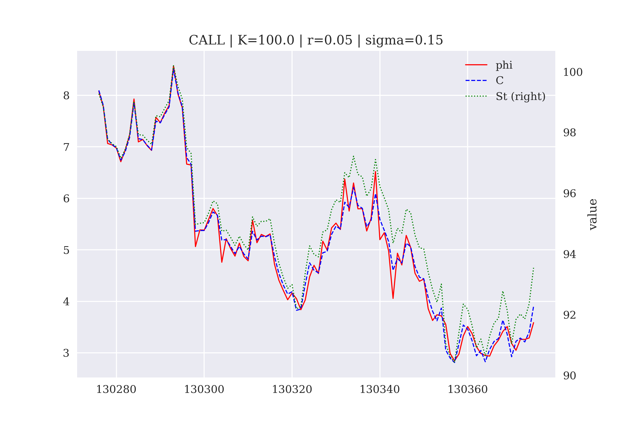
Figure 25. Option and replication portfolio values compared

Histogram of the replication errors shows the histogram of the replication errors for that particular test run.

In [114]: hedgingagent.env.portfolios[
              hedgingagent.env.portfolios['e'] == n]['p&l[$]'].hist(
                  bins=35, color='blue')
          plt.title(title)
          plt.xlabel('P&L')
          plt.ylabel('frequency');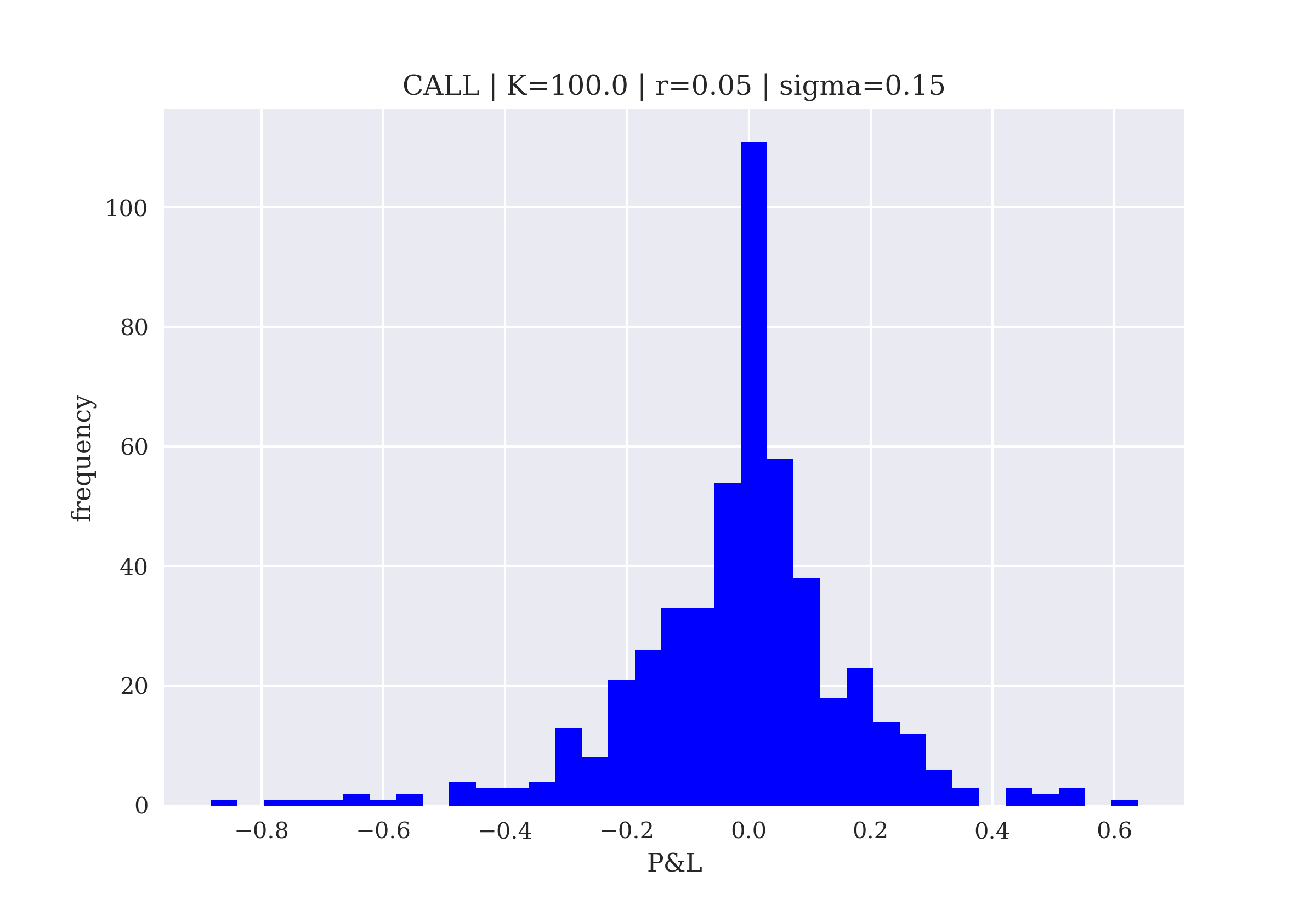

Figure 26. Histogram of the replication errors

7.4. Conclusions

Dynamic hedging and option replication are key methods in mathematical finance for the pricing and risk management of options and other derivative instruments. Generally, for their implementation, these methods rely on a specific financial model that relates relevant model (market) parameters with the value of the derivative instrument at hand. This chapter shows that DQL as an algorithm can learn almost perfect replication strategies based on interacting with a hedging environment that only provides a parsimonious set of parameters and values but no information about the financial model or the actual delta of the option.

While previous chapters focus on discrete action spaces, the hedging problem in this chapter represents an optimal control problem in that the action to be chosen is a stock position that can take on any value between zero and one. To this end, the DNN of the DQL agent predicts the total reward for a specific replication portfolio given a certain state of the hedging environment. The agent chooses the action with the highest predicted total reward. In the case of the hedging problem of this chapter, the agent minimizes the total penalty which is driven by the replication errors that the agent’s strategy generates over the single steps.

All in all, the hedging agent learns dynamic option replication in a remarkably good fashion. The observed replication errors are pretty small and on average close to zero.

7.5. References

Books and articles cited in this chapter:

Baxter, Martin and Andrew Rennie (1996): Financial Calculus—An Introduction to Derivative Pricing. Cambridge University Press, Cambridge.
Black, Fischer and Myron Scholes (1973): “The Pricing of Options and Corporate Liabilities.” Journal of Political Economy, Vol. 81, No. 3, 638–659.
Duffie, Darrell (1998): “Black, Merton and Scholes: Their Central Contributions to Economics.” The Scandinavian Journal of Economics, Vol. 100, No. 2, 411-423.
Hilpisch, Yves (2015): Derivatives Analytics with Python. Wiley Finance, Chichester.
Maney, Kevin (2017): “Goldman Sacked: How AI Will Transform Wall Street.” Newsweek, 10. March 2017.
Merton, Robert (1973): “Theory of Rational Option Pricing.” Bell Journal of Economics and Management Science, Vol. 4, No. 1, 141–183.
Taleb, Nassim (1996): Dynamic Hedging: Managing Vanilla and Exotic Options. John Wiley & Sons, New York et al.
Timmermann, Allan and Clive Granger (2004): “Efficient Market Hypothesis and Forecasting.” International Journal of Forecasting, Vol. 20, 15-27.

7.6. BSM (1973) Formula

The following Python code implements the BSM73 European call option pricing formula as introduced in Delta Hedging:

#
# Valuation of European call options
# in Black-Scholes-Merton (1973) model
#
# (c) Dr. Yves J. Hilpisch
# Reinforcement Learning for Finance
#

from math import log, sqrt, exp
from scipy import stats


def bsm_call_value(St, K, T, t, r, sigma):
    ''' Valuation of European call option in BSM model.
    Analytical formula.

    Parameters
    ==========
    St: float
        stock/index level at date/time t
    K: float
        fixed strike price
    T: float
        maturity date/time (in year fractions)
    t: float
        current data/time
    r: float
        constant risk-free short rate
    sigma: float
        volatility factor in diffusion term

    Returns
    =======
    value: float
        present value of the European call option
    '''
    St = float(St)
    d1 = (log(St / K) + (r + 0.5 * sigma ** 2) * (T - t)) / (sigma * sqrt(T - t))
    d2 = (log(St / K) + (r - 0.5 * sigma ** 2) * (T - t)) / (sigma * sqrt(T - t))
    # stats.norm.cdf --> cumulative distribution function
    #                    for normal distribution
    value = (St * stats.norm.cdf(d1, 0, 1) -
             K * exp(-r * (T - t)) * stats.norm.cdf(d2, 0, 1))
    return value

8. Dynamic Asset Allocation

Professional gamblers, who have to have an advantage, speak of “money management.” This refers to the tricky and all-important issue of how to achieve the greatest profit from a favorable betting opportunity. You can be the world’s greatest poker player, backgammon player, or handicapper, but if you can’t manage your money, you’ll end up broke. The sad fact is, almost everyone who gambles goes broke in the long run.

— Poundstone (2010)

The world economy has grown at a decent enough clip over the past two decades, at more than 3% a year. Yet it has been left in the dust by growth in wealth. Between 2000 and 2020 the total stock rose from $160trn, or four times global output, to $510trn, or six times output.

— The Economist (2023)

The challenge of asset allocation is a major problem in the financial domain, underscored by the vast amounts of money that individuals and institutions must invest. It is also a problem that started the quantitative revolution in finance with the seminal work of Markowitz (1952) on “Portfolio Selection”. In this paper, Markowitz proposes a purely statistical approach for composing portfolios as compared to, say, the fundamental analysis of companies and their stocks.

While the early work in this regard focuses on the static, or non-repeated, problem of allocating funds across different assets, a more realistic way of approaching asset allocation is in its dynamic, or repeated, form. Like algorithmic trading and dynamic hedging, dynamic asset allocation is a problem that fits well into the general framework of dynamic programming as introduced in Financial Q-Learning. Therefore, it is a problem that can also be tackled with deep Q-learning (DQL) to arrive at approximate, numerical solutions. The paper by Merton (1969) represents an early work about dynamic asset allocation in a continuous-time model where uncertainty is generated by geometric Brownian motion. He uses dynamic programming and the Bellman principle to derive optimal solutions for several special cases, including a simple two-asset case and a more realistic multiple-asset case with an infinite horizon.

This chapter addresses three cases for dynamically allocating assets. In the first case, covered in Two-Fund Separation, two assets, a risky and a riskless one, are available for investment. Two-Asset Case covers the case of two risky assets. Against this background, Three-Asset Case adds a third risky asset to the investment set. From three assets, the generalization to four or more assets is straightforward. Finally, Equally Weighted Portfolio compares the results in the three-asset case against the performance of an equally weighted portfolio.

8.1. Two-Fund Separation

The concept of two-fund separation dates back to Markowitz (1952). It states that in equilibrium and under certain assumptions, financial market investors will hold a combination of the riskless asset and the risky market portfolio — and nothing else. The market portfolio lies on the efficient frontier of the set of achievable risk-return combinations. The efficient frontier represents all those portfolios that give the maximum expected return for a given level of risk. In practical applications, the market portfolio, which is not directly investable, is generally approximated by a broad stock market index such as the S&P 500. The straight line connecting the riskless asset and the market portfolio in risk-return space is generally called the capital market line (CML). For more details on this and related topics, see also chapter 5 of Copeland, Weston, and Shastri (2005).

Based on some simple numerical assumptions, the following Python code illustrates the CML visually. The usual imports and customization first:

In [1]: import math
        import random
        import numpy as np
        import pandas as pd
        from scipy import stats
        from pylab import plt, mpl

In [2]: plt.style.use('seaborn-v0_8')
        mpl.rcParams['figure.dpi'] = 300
        mpl.rcParams['savefig.dpi'] = 300
        mpl.rcParams['font.family'] = 'serif'
        np.set_printoptions(suppress=True)
        pd.set_option('display.float_format', lambda x: '%.3f' % x)

Capital market line (CML) shows an illustration of the CML. Without short selling, an investor can achieve any risk-return combination on the line that connects the riskless asset (triangle) with the market portfolio (thick dot). If short selling is allowed, combinations to the right of the market portfolio are also achievable. Those portfolios would represent leveraged positions in the market portfolio, that is, a combination of a short position in the riskless asset and a long position in the market portfolio that is greater than 100% of the investable capital. All in all, the CML embodies one of the fundamental concepts in finance: an investor who is willing to bear more risk, can expect — everything else being equal — a higher return on their investment.

In [3]: r = 0.025  (1)
        beta = 0.2  (2)
        sigma = 0.375  (3)
        mu = r + beta * sigma  (4)
        mu  (4)
Out[3]: 0.1

In [4]: vol = np.linspace(0, 0.5)  (5)
        ret = r + beta * vol  (5)

In [5]: fig, ax = plt.subplots()
        plt.plot(vol, ret, 'b', label='capital market line (CML)')
        plt.plot(0, r, 'g^', label='riskless asset')
        plt.plot(sigma, mu, 'ro', label='market portfolio')
        plt.xlabel('volatility/risk')
        plt.ylabel('expected return')
        ax.set_xticks((0, sigma))
        ax.set_xticklabels((0, '$\sigma$',))
        ax.set_yticks((0, r, mu))
        ax.set_yticklabels((0, '$r$', '$\mu$'))
        plt.ylim(0, 0.15)
        plt.legend();

1	The return of the riskless asset.
2	The slope of the capital market line.
3	The volatility of the market portfolio.
4	The expected return of the market portfolio.
5	The risk-return combinations to be plotted.

Figure 27. Capital market line (CML)

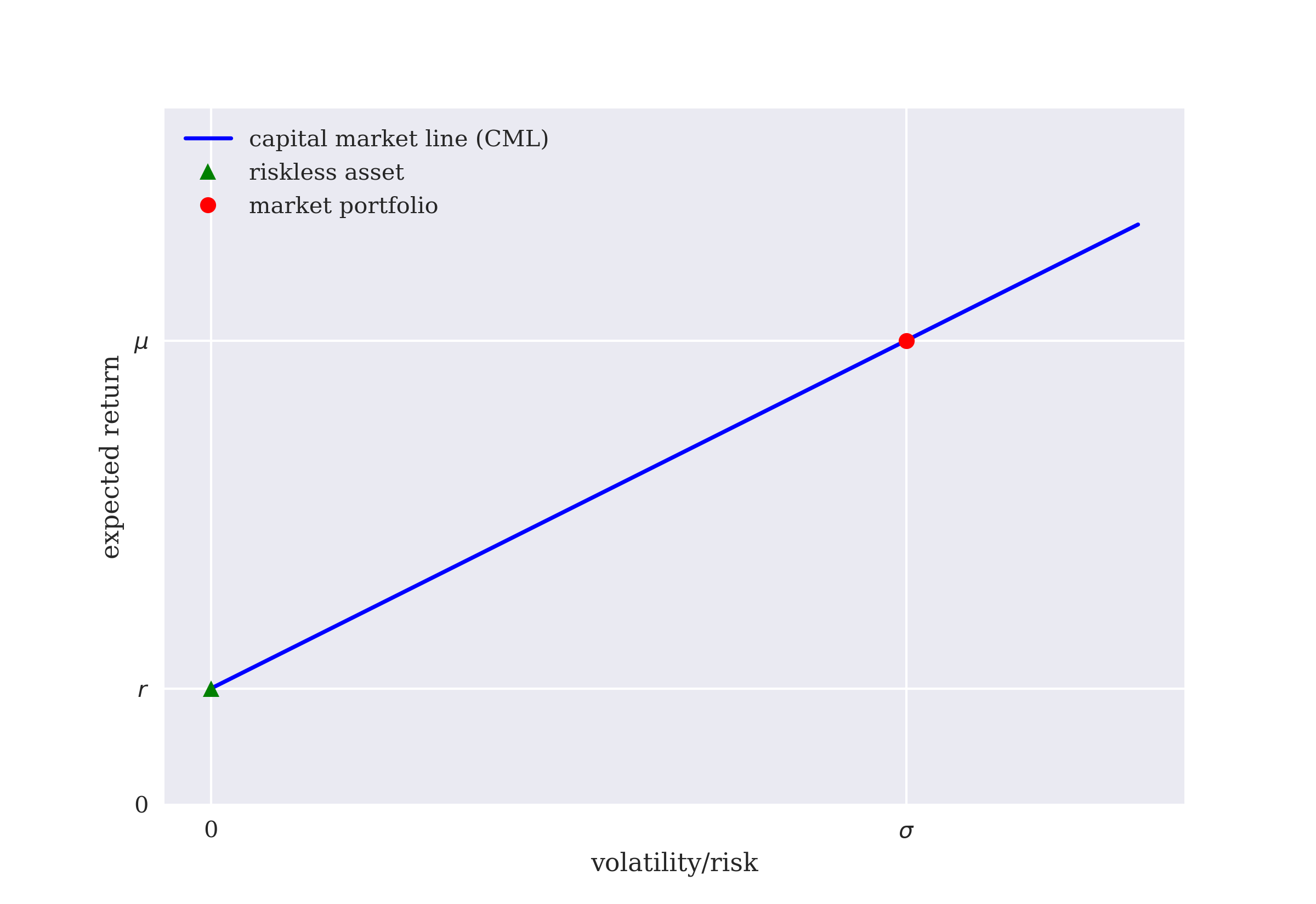
60/40 Portfolios

A popular investment strategy, proposed for decades by the asset management industry and academia, is the so-called “60/40 portfolio” which allocates 60% of a portfolio to stocks and 40% to bonds. Although bonds are not riskless in general, the idea is similar to two-fund separation. The addition of less risky bonds to a stock portfolio reduces the overall risk of that portfolio while preserving the long-term upside potential of the stock market through a larger allocation to stocks. It has also often been observed that bond prices and stock prices are negatively correlated which can further reduce portfolio risk. These characteristics should especially appeal to a “moderate risk investor”. However, in 2022, for example, this kind of portfolio has performed poorly, mainly driven by fast-rising interest rates. For more background and details refer to the commentary by Chisholm (2023) which also presents performance data over multiple decades.

In what follows, a DQL agent is trained to invest in the two types of assets. The riskless asset simply yields a fixed return. The risky asset is modeled as a geometric Brownian motion (GBM) as in Merton (1969), Black and Scholes (1973), and Merton (1973). The approach in this section is similar to the one used in Dynamic Hedging. Therefore, the Investing environment developed step-by-step in what follows resembles the Hedging environment. As before, two helper classes are used. The agent can choose the position in the risky asset from the unit interval. “0” means no investment in the risky asset, “1” means 100% investment in it. The difference to 1 or 100% is invested in the riskless asset:

In [6]: class observation_space:
            def __init__(self, n):
                self.shape = (n,)

In [7]: class action_space:
            def __init__(self, n):
                self.n = n

            def seed(self, seed):
                random.seed(seed)

            def sample(self):
                return random.random()  (1)

1	Samples a random action (stock investment) from the unit interval.

As in the dynamic hedging case, the Investing environment takes multiple parameters as input for the simulation of the GBM. It also keeps track of the initial balance and the two most recent portfolio values:

In [8]: class Investing:
            def __init__(self, S0, T, r_, mu_, sigma_, steps, amount):
                self.initial_value = S0
                self.maturity = T
                self.short_rate_ = r_  (1)
                self.index_drift_ = mu_  (1)
                self.volatility_ = sigma_  (1)
                self.steps = steps
                self.initial_balance = amount  (2)
                self.portfolio_value = amount  (3)
                self.portfolio_value_new = amount  (4)
                self.observation_space = observation_space(4)
                self.osn = self.observation_space.shape[0]
                self.action_space = action_space(1)
                self._generate_data()
                self.portfolios = pd.DataFrame()
                self.episode = 0

1	The parameters can be passed as iterable objects with multiple values.
2	The initial investment is stored.
3	The current portfolio value is initialized.
4	The new portfolio value is initialized.

The next method simulates the paths for the risky asset (X) and calculates the values for the riskless asset (Y):

In [9]: class Investing(Investing):
            def _generate_data(self):
                s = [self.initial_value]
                self.short_rate = random.choice(self.short_rate_)  (1)
                self.index_drift = random.choice(self.index_drift_)  (1)
                self.volatility = random.choice(self.volatility_)  (1)
                self.dt = self.maturity / self.steps
                for t in range(1, self.steps + 1):
                    st = s[t - 1] * math.exp(
                        (self.index_drift * self.dt +
                          self.volatility * math.sqrt(self.dt) * random.gauss(0, 1))
                    )  (2)
                    s.append(st)
                self.data = pd.DataFrame(s, columns=['Xt'])
                self.data['Yt'] = self.initial_value * np.exp(
                    self.short_rate * np.arange(len(self.data)) * self.dt)  (3)

1	Randomly selects the parameter values.
2	Simulates the risky asset path.
3	Calculates the riskless asset values.

The following methods only require minor adjustments compared to the Hedging environment:

In [10]: class Investing(Investing):
             def _get_state(self):
                 Xt = self.data['Xt'].iloc[self.bar]
                 Yt = self.data['Yt'].iloc[self.bar]
                 return np.array([Xt, Yt, self.xt, self.yt]), {}

             def seed(self, seed=None):
                 if seed is not None:
                     random.seed(seed)

             def reset(self):
                 self.bar = 0
                 self.xt = 0
                 self.yt = 0
                 self.treward = 0
                 self.portfolio_value = self.initial_balance
                 self.portfolio_value_new = self.initial_balance
                 self.episode += 1
                 self._generate_data()
                 self.state, _ = self._get_state()
                 return self.state, _

With the final two methods, the Python class for the Investing environment is complete. The .add_results() method allows the collection of relevant data points for all episodes and steps. This simplifies further analyses of the results after the learning and testing phases:

In [11]: class Investing(Investing):
             def add_results(self, pl):
                 df = pd.DataFrame({'e': self.episode, 'xt': self.xt,
                            'yt': self.yt, 'pv': self.portfolio_value,
                            'pv_new': self.portfolio_value_new, 'p&l[$]': pl,
                            'p&l[%]': pl / self.portfolio_value_new,
                            'Xt': self.state[0],  'Yt': self.state[1],
                            'Xt_new': self.new_state[0],
                            'Yt_new': self.new_state[1],
                            'r': self.short_rate, 'mu': self.index_drift,
                            'sigma': self.volatility}, index=[0])
                 self.portfolios = pd.concat((self.portfolios, df),
                                             ignore_index=True)

             def step(self, action):
                 self.bar += 1
                 self.new_state, _ = self._get_state()
                 if self.bar == 1:  (1)
                     self.xt = action (2)
                     self.yt = (1 - action) (3)
                     pl = 0.
                     reward = 0.
                     self.add_results(pl)
                 else:
                     self.portfolio_value_new = (
                         self.xt * self.portfolio_value *
                         self.new_state[0] / self.state[0] +
                         self.yt * self.portfolio_value *
                         self.new_state[1] / self.state[1])  (4)
                     pl = self.portfolio_value_new - self.portfolio_value  (5)
                     self.xt = action (6)
                     self.yt = (1 - action) (7)
                     self.add_results(pl)  (8)
                     reward = pl  (9)
                     self.portfolio_value = self.portfolio_value_new  (10)
                 if self.bar == len(self.data) - 1:
                     done = True
                 else:
                     done = False
                 self.state = self.new_state
                 return self.state, reward, done, False, {}

1	The initial action is treated separately.
2	The position for the risky asset is set.
3	The position for the riskless asset is set.
4	The new portfolio value is calculated given the previous asset allocation.
5	The profit or loss (P&L) is calculated in absolute terms.
6	The position for the risky asset is updated.
7	The position for the riskless asset is updated.
8	The results are added to the `DataFrame`.
9	The reward is set to the P&L.
10	The portfolio value is updated.

Next, consider the following parametrization for the environment, including a fixed seed value for the random number generator. Value paths for the riskless and risky asset shows the evolution of the values of the two assets. Here, the initial value is set to 1 for both assets:

In [12]: S0 = 1.

In [13]: investing = Investing(S0=S0, T=1.0, r_=[0.05], mu_=[0.3],
                       sigma_=[0.35], steps=252, amount=1)

In [14]: investing.seed(750)

In [15]: investing._generate_data()

In [16]: investing.data.plot(style=['g--', 'b:'], lw=1.0)
         plt.xlabel('time step')
         plt.ylabel('price');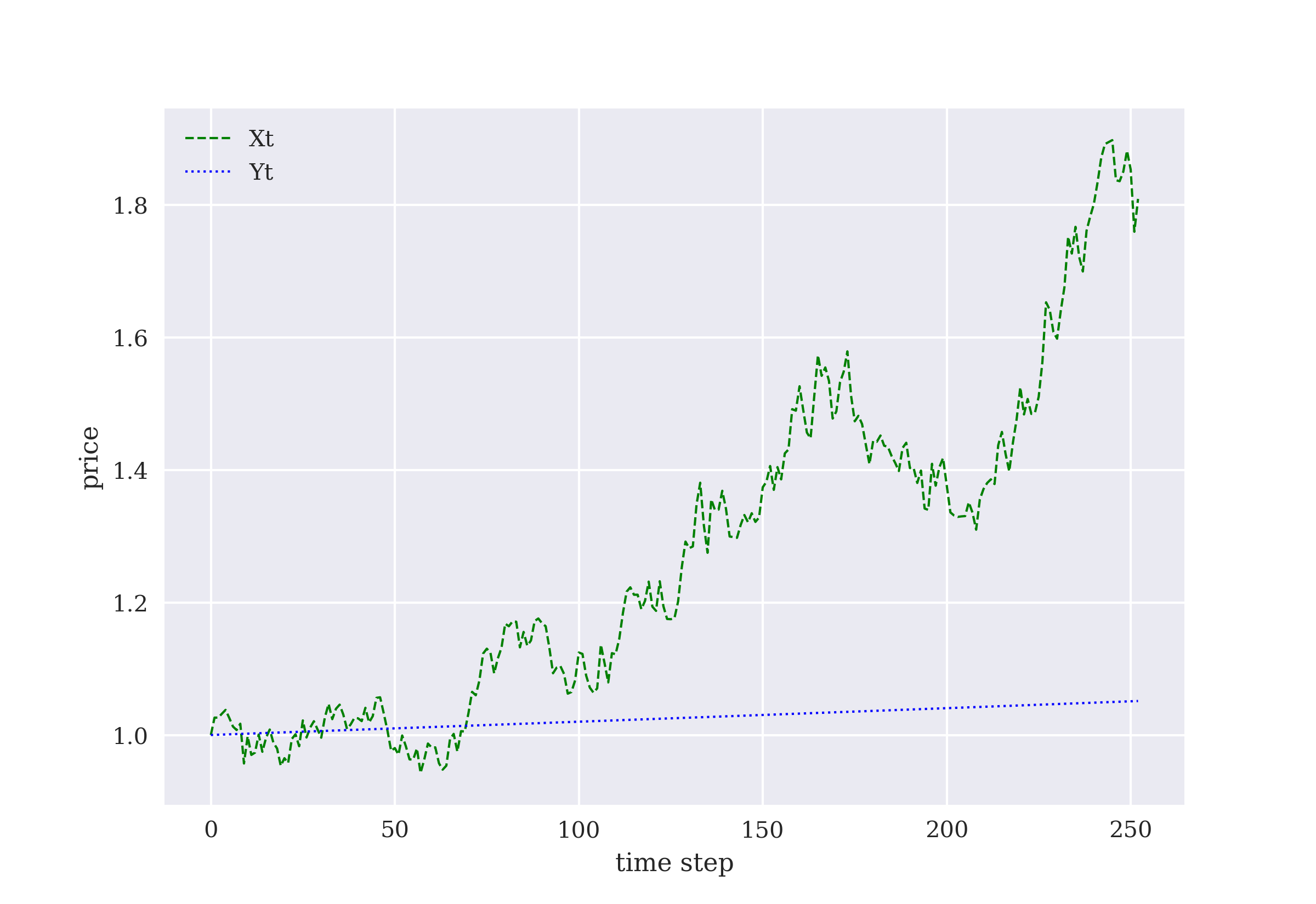

Figure 28. Value paths for the riskless and risky asset

The following Python code lets a random agent interact with the environment. Portfolio values for the random agent shows the relative performance of the portfolio value compared to the value paths of the riskless and the risky assets. Given the random allocation of the agent and the negative overall performance of the risky asset, the random strategy outperforms both the riskless and the risky asset in the case shown in the figure:

In [17]: investing.reset()
Out[17]: (array([1., 1., 0., 0.]), {})

In [18]: for _ in range(investing.steps - 1):
             investing.step(investing.action_space.sample())

In [19]: investing.portfolios.head().round(3)
Out[19]:    e    xt    yt    pv  pv_new  p&l[$]  p&l[%]    Xt    Yt  Xt_new  Yt_new  \
         0  1 0.587 0.413 1.000   1.000   0.000   0.000 1.000 1.000   0.980   1.000
         1  1 0.001 0.999 1.000   1.009   0.009   0.009 0.980 1.000   0.994   1.000
         2  1 0.838 0.162 1.009   1.009   0.000   0.000 0.994 1.000   0.974   1.001
         3  1 0.981 0.019 1.009   0.998  -0.011  -0.011 0.974 1.001   0.962   1.001
         4  1 0.167 0.833 0.998   0.979  -0.020  -0.020 0.962 1.001   0.943   1.001

               r    mu  sigma
         0 0.050 0.300  0.350
         1 0.050 0.300  0.350
         2 0.050 0.300  0.350
         3 0.050 0.300  0.350
         4 0.050 0.300  0.350

In [20]: investing.portfolios[['Xt', 'Yt', 'pv']].plot(
             title='PORTFOLIO VALUE | RANDOM AGENT',
             style=['g--', 'b:', 'r-'], lw=1)
         plt.xlabel('time step')
         plt.ylabel('value');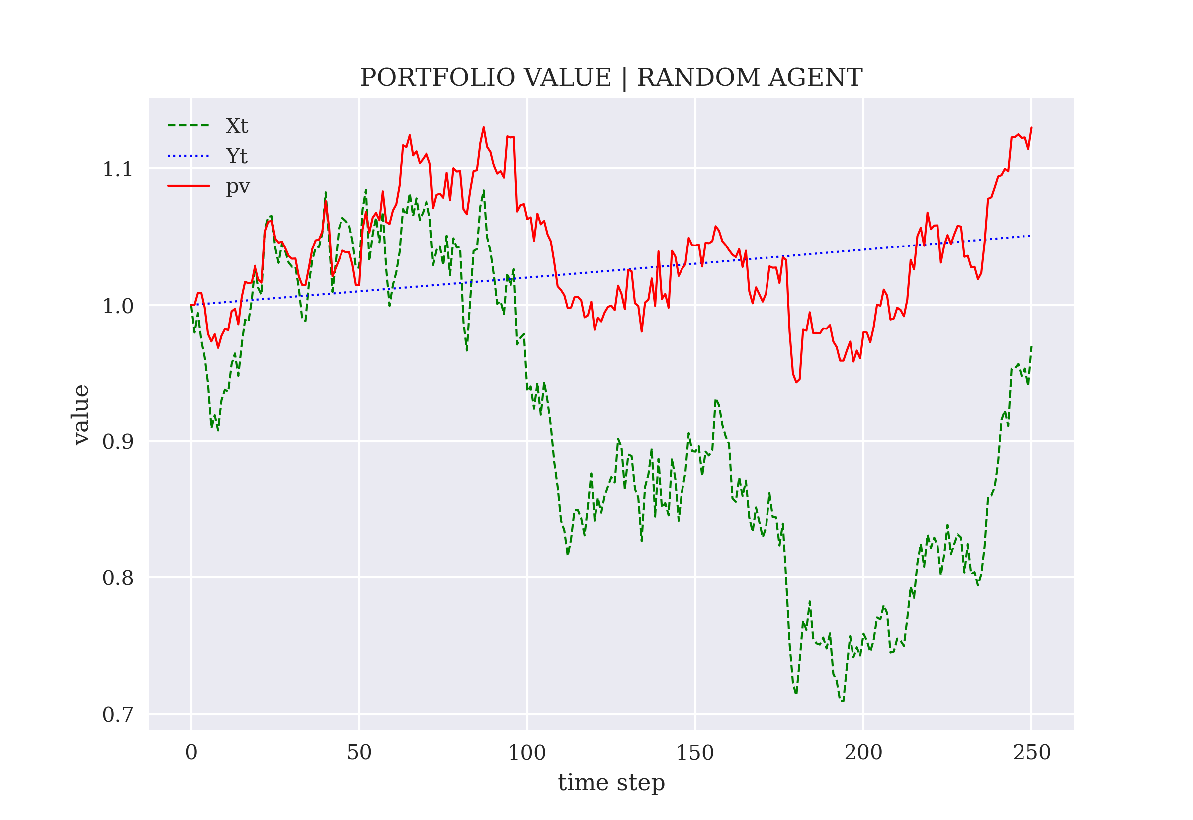

Figure 29. Portfolio values for the random agent

As in the previous chapter, the InvestingAgent class inherits from the DQLAgent class as presented in DQLAgent Class. The neural network takes as input the four values that represent the state of the environment and the asset allocation — the value of the risky asset, the value of the riskless asset, the position in the risky asset, and the position in the riskless asset. It gives as output a single, floating-point value. The output represents the expected reward given the state of the environment and the asset allocation.

In [21]: from dqlagent import *

In [22]: opt = keras.optimizers.legacy.Adam

In [23]: class InvestingAgent(DQLAgent):
             def _create_model(self, hu, lr):
                 self.model = Sequential()
                 self.model.add(Dense(hu, input_dim=self.n_features,
                                 activation='relu'))
                 self.model.add(Dense(hu, activation='relu'))
                 self.model.add(Dense(1, activation='linear'))  (1)
                 self.model.compile(loss='mse',
                         optimizer=opt(learning_rate=lr))

1	Linear floating-point valued output.

As in the dynamic hedging case, the optimal action is derived through numerical optimization. The .opt_action() method gives the allocation for the risky asset that yields the maximal expected reward. The allocation for the riskless asset follows by definition:

In [24]: from scipy.optimize import minimize

In [25]: class InvestingAgent(InvestingAgent):
             def opt_action(self, state):
                 bnds = [(0, 1)]  (1)
                 def f(state, x):  (2)
                     s = state.copy()
                     s[0, self.xp] = x  (3)
                     s[0, self.yp] = 1 - x  (4)
                     return self.model.predict(s)[0, 0]  (5)
                 action = minimize(lambda x: -f(state, x), 0.5,
                                 bounds=bnds, method='Nelder-Mead',
                                 )['x'][0]  (6)
                 return action

             def act(self, state):
                 if random.random() <= self.epsilon:
                     return self.env.action_space.sample()
                 action = self.opt_action(state)  (7)
                 return action

1	The bounds for the allocation in the risky asset.
2	The function `f()` to be maximized.
3	Sets the risky asset allocation to the input value `x`.
4	Sets the riskless asset allocation to `1 - x`.
5	Predicts the expected reward from the neural network.
6	Maximizes the expected reward by minimizing `-f()`.

Similarly, the .replay() method predicts the expected future reward based on the allocation to the risky asset:

In [26]: class InvestingAgent(InvestingAgent):
             def replay(self):
                 batch = random.sample(self.memory, self.batch_size)
                 for state, action, next_state, reward, done in batch:
                     ns = next_state.copy()
                     target = reward
                     if not done:
                         action = self.opt_action(ns)  (1)
                         ns[0, self.xp] = action  (2)
                         ns[0, self.yp] = 1 - action  (3)
                         target += (self.gamma *
                             self.model.predict(ns)[0, 0])  (4)
                     self.model.fit(state, np.array([target]),
                                    epochs=1, verbose=False)
                 if self.epsilon > self.epsilon_min:
                     self.epsilon *= self.epsilon_decay

1	Generates the optimal action as the allocation in the risky asset.
2	Updates the allocation to the risky asset.
3	Updates the allocation to the riskless asset.
4	Calculates and adds the discounted, delayed reward.

Finally, the following Python code adjusts the .testing() methods to reflect the new setup. The major change is the call of the .opt_action() method to retrieve optimal asset allocations for the risky asset:

In [27]: class InvestingAgent(InvestingAgent):
             def test(self, episodes, verbose=True):
                 for e in range(1, episodes + 1):
                     state, _ = self.env.reset()
                     state = self._reshape(state)
                     treward = 0
                     for _ in range(1, len(self.env.data) + 1):
                         action = self.opt_action(state)
                         state, reward, done, trunc, _ = self.env.step(action)
                         state = self._reshape(state)
                         treward += reward
                         if done:
                             templ = f'episode={e} | '
                             templ += f'total reward={treward:4.2f}'
                             if verbose:
                                 print(templ, end='\r')
                             break

Consider now the Investing environment initialized with several values for the short rate, the expected return (drift), and the volatility of the risky asset. The InvestingAgent is trained on a larger number of simulations for randomly chosen parameter combinations:

In [28]: def set_seeds(seed=500):
             random.seed(seed)
             np.random.seed(seed)
             tf.random.set_seed(seed)

In [29]: set_seeds()

In [30]: investing = Investing(S0=S0, T=1.0, r_=[0, 0.025, 0.05],
                       mu_=[0.05, 0.1, 0.15],
                       sigma_=[0.1, 0.2, 0.3], steps=252, amount=1)

In [31]: agent = InvestingAgent('2FS', feature=None, n_features=4,
                              env=investing, hu=128, lr=0.00025)

In [32]: agent.xp = 2  (1)
         agent.yp = 3  (2)

In [33]: episodes = 64

In [34]: %time agent.learn(episodes)
         episode=  64 | treward=  0.281 | max=  0.360
         CPU times: user 29.6 s, sys: 4.7 s, total: 34.3 s
         Wall time: 28.9 s

In [35]: agent.epsilon
Out[35]: 0.8519730927255319

1	Sets the index position for the risky asset.
2	Sets the index position for the riskless asset.

Then, the agent is tested for a larger number of test runs as well. For a single test run, Portfolio values for the InvestingAgent shows the evolution of the portfolio value given the asset allocation as chosen by the agent:

In [36]: agent.env.portfolios = pd.DataFrame()

In [37]: %time agent.test(10)
         CPU times: user 18.1 s, sys: 2.74 s, total: 20.8 s
         Wall time: 17.3 s

In [38]: n = max(agent.env.portfolios['e'])  (1)

In [39]: res = agent.env.portfolios[agent.env.portfolios['e'] == n]
         res.head()
Out[39]:        e    xt    yt    pv  pv_new  p&l[$]  p&l[%]    Xt    Yt  Xt_new  \
         2268  74 0.598 0.402 1.000   1.000   0.000   0.000 1.000 1.000   1.002
         2269  74 0.598 0.402 1.000   0.999  -0.001  -0.001 1.002 1.000   1.001
         2270  74 0.598 0.402 0.999   1.007   0.008   0.008 1.001 1.000   1.014
         2271  74 0.596 0.404 1.007   1.010   0.003   0.003 1.014 1.001   1.019
         2272  74 0.592 0.408 1.010   1.017   0.006   0.006 1.019 1.001   1.029

               Yt_new     r    mu  sigma
         2268   1.000 0.050 0.150  0.100
         2269   1.000 0.050 0.150  0.100
         2270   1.001 0.050 0.150  0.100
         2271   1.001 0.050 0.150  0.100
         2272   1.001 0.050 0.150  0.100

In [40]: p = res.iloc[0][['r', 'mu', 'sigma']]

In [41]: t = f"r={p['r']} | mu={p['mu']} | sigma={p['sigma']}"

In [42]: res[['Xt', 'Yt', 'pv']].plot(
             title='PORTFOLIO VALUE | ' + t,
             style=['g--', 'b:', 'r-'], lw=1)
         plt.xlabel('time step')
         plt.ylabel('value');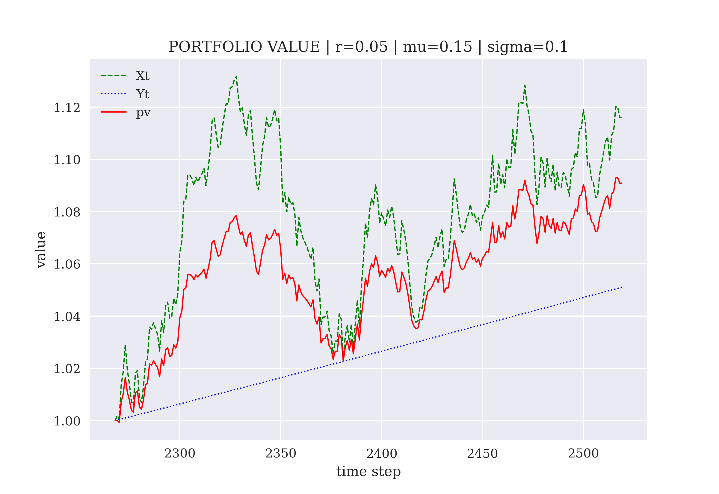

Figure 30. Portfolio values for the InvestingAgent

It is interesting to investigate some statistics in this context. In this particular test run, the 60/40 strategy is almost exactly dynamically implemented by the agent (see Dynamic allocation to the risky asset (in percent)). While the return of the agent’s strategy is between the riskless and the risky asset, the resulting Sharpe ratio of the agent’s 60/40 strategy is higher than the one of the risky asset^[23]:

In [43]: rets = res[['Xt', 'Yt', 'pv']].pct_change(
             ).mean() / agent.env.dt  (1)
         rets
Out[43]: Xt   0.115
         Yt   0.050
         pv   0.089
         dtype: float64

In [44]: stds = res[['Xt', 'Yt', 'pv']].pct_change(
             ).std() / math.sqrt(agent.env.dt)  (2)
         stds
Out[44]: Xt   0.102
         Yt   0.000
         pv   0.059
         dtype: float64

In [45]: rets[['Xt', 'pv']] / stds[['Xt', 'pv']]  (3)
Out[45]: Xt   1.128
         pv   1.510
         dtype: float64

In [46]: res['xt'].mean()  (4)
Out[46]: 0.5752329024057541

In [47]: res['xt'].std()  (5)
Out[47]: 0.012903089308493553

In [48]: res['xt'].plot(title='RISKY ALLOCATION | ' + t,
                        lw=1.0, c='b')
         plt.ylim(res['xt'].min() - 0.1, res['xt'].max() + 0.1)
         plt.xlabel('time step');

1	Calculates the annualized mean returns.
2	Calculates the annualized volatilities.
3	Derives the Sharpe ratios.
4	Average risky asset allocation.
5	Standard deviation of that allocation.

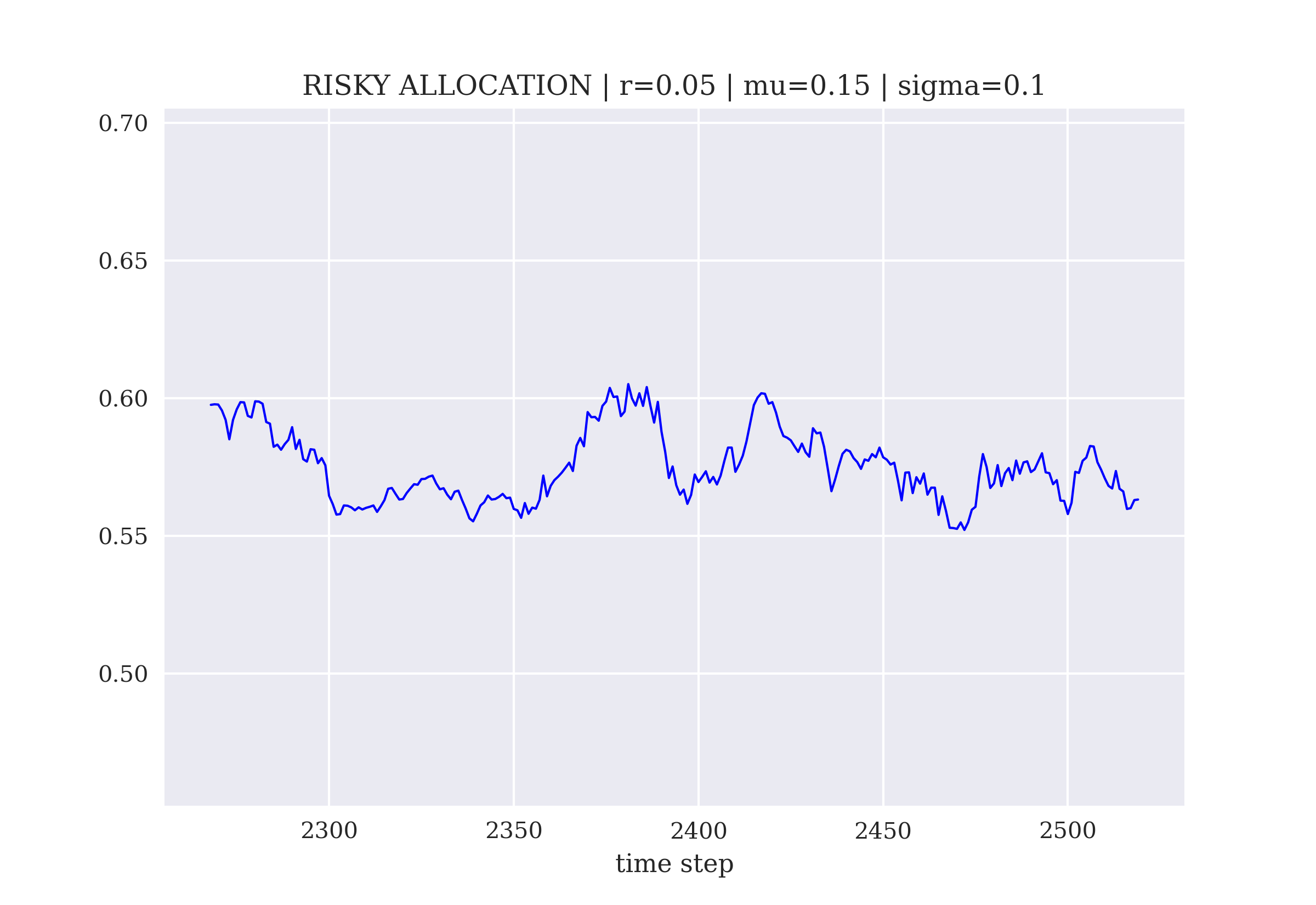
Figure 31. Dynamic allocation to the risky asset (in percent)

The following shows several statistics with regard to the allocation in the risky asset (xt). Basically independent of the drift and risk parameters, the risky allocation is around 60% on average with maximum values of around 75%.

In [49]: agent.env.portfolios.groupby('mu')['xt'].describe()
Out[49]:          count  mean   std   min   25%   50%   75%   max
         mu
         0.050  504.000 0.600 0.038 0.552 0.582 0.599 0.605 0.730
         0.100 1008.000 0.595 0.080 0.423 0.566 0.587 0.602 0.749
         0.150 1008.000 0.603 0.051 0.427 0.573 0.592 0.600 0.747

In [50]: agent.env.portfolios.groupby('sigma')['xt'].describe()
Out[50]:          count  mean   std   min   25%   50%   75%   max
         sigma
         0.100 1260.000 0.581 0.015 0.552 0.568 0.580 0.597 0.615
         0.200  756.000 0.623 0.059 0.427 0.592 0.600 0.610 0.747
         0.300  504.000 0.610 0.110 0.423 0.563 0.599 0.723 0.749

Similarly, the following data provides the same statistics for the portfolio values over time. Apart from the case with the highest risk factor, the portfolios are above 1 on average. Overall, one can say, that they vary not that much on average for the different parameter values:

In [51]: agent.env.portfolios.groupby('mu')['pv_new'].describe()
Out[51]:          count  mean   std   min   25%   50%   75%   max
         mu
         0.050  504.000 1.029 0.036 0.945 1.003 1.022 1.051 1.123
         0.100 1008.000 1.016 0.089 0.833 0.951 1.030 1.080 1.194
         0.150 1008.000 1.028 0.036 0.916 1.003 1.025 1.058 1.104

In [52]: agent.env.portfolios.groupby('sigma')['pv_new'].describe()
Out[52]:          count  mean   std   min   25%   50%   75%   max
         sigma
         0.100 1260.000 1.056 0.044 0.986 1.022 1.049 1.080 1.194
         0.200  756.000 1.017 0.037 0.916 0.989 1.013 1.040 1.123
         0.300  504.000 0.953 0.072 0.833 0.888 0.951 1.008 1.140

To close this section, another analysis of the test run sheds more light on how the agent behaves. The agent reduces the exposure to the risky asset in cases when the price of it rises. It does the opposite in cases when its price falls. However, the risky allocation remains throughout between 55% and 60%. One could call such a strategy a negative feedback strategy (see Portfolio values and dynamic allocation to the risky asset). The agent achieves a performance well above the risk-less return and even close to the return of the risky asset:

In [53]: n = max(agent.env.portfolios['e'])  (1)

In [54]: res = agent.env.portfolios[agent.env.portfolios['e'] == n]

In [55]: p = res.iloc[0][['r', 'mu', 'sigma']]

In [56]: t = f"r={p['r']} | mu={p['mu']} | sigma={p['sigma']}"

In [57]: ax = res[['Xt', 'Yt', 'pv', 'xt']].plot(
             title='PORTFOLIO VALUE | ' + t,
             style=['g--', 'b:', 'r-', 'm-.'], lw=1,
             secondary_y='xt'
         )

1	Selects the test run.

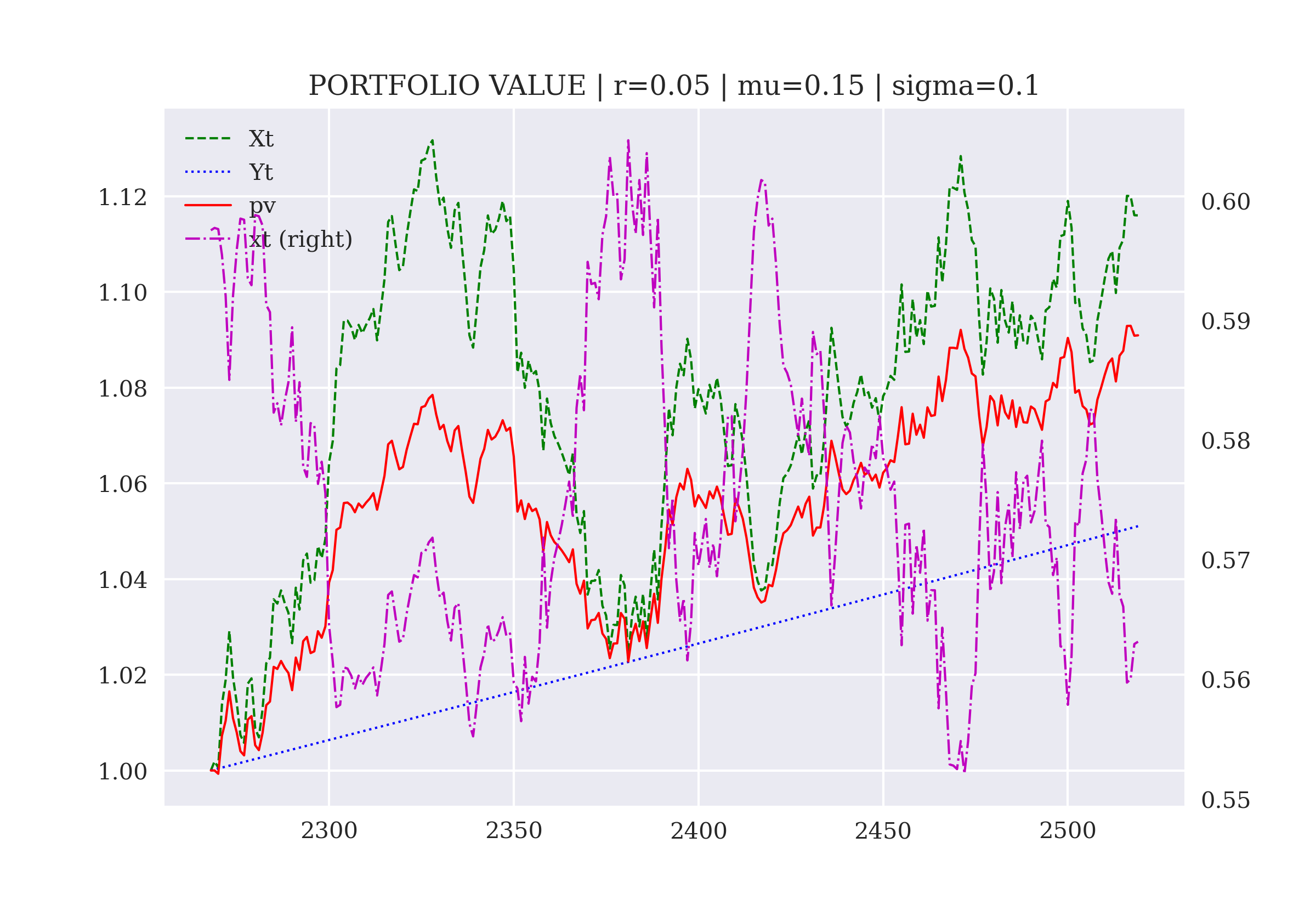
Figure 32. Portfolio values and dynamic allocation to the risky asset

8.2. Two-Asset Case

The analysis of the previous section can easily be adjusted to include two risky assets. This section is based on real historical data for a number of different financial instruments. The analysis focuses on data for the S&P 500 stock index and the VIX volatility index. The time series of the index levels are known to be highly negatively correlated. Investment strategies that keep the fractions of the two constant over time are known to yield superior returns as compared to other investment strategies involving these two assets. Such strategies are called constant proportion investment strategies. Such a strategy uses dynamic portfolio re-balancing to keep the proportions invested in each security at roughly the same level, say 60% for the S&P 500 and 40% in the VIX.^[24]

Strategy Implementation

This section makes the simplifying assumption that both the S&P 500 and the VIX are tradable assets. In practice, this is not the case, and other financial instruments that rely on such indices are needed. For example, one can use an exchange-traded fund based on the S&P 500 as a proxy for the stock index. Futures or options on the index could also be used. Similarly, one can use futures and options written on the VIX index as proxies for the volatility index. In particular, when using futures and options this involves a number of implementation-related topics — such as roll-overs of the derivatives positions — that are ignored in this section. Other simplifying assumptions, such as zero transaction costs, are also made implicitly.

Although there are a number of adjustments to be made to the Investing environment from the previous section, they are all straightforward and should all be easy to understand. The new Investing class allows for the selection of two risky assets. For these, a random, contiguous subset is selected from the original data set. The data set itself is the same as the one used in Financial Q-Learning for the Finance environment class:

In [58]: class Investing(Investing):
             def __init__(self, asset_one='.SPX', asset_two='.VIX',
                          steps=252, amount=1):
                 self.asset_one = asset_one
                 self.asset_two = asset_two
                 self.steps = steps
                 self.initial_balance = amount
                 self.portfolio_value = amount
                 self.portfolio_value_new = amount
                 self.observation_space = observation_space(4)
                 self.osn = self.observation_space.shape[0]
                 self.action_space = action_space(1)
                 self.retrieved = False
                 self._generate_data()
                 self.portfolios = pd.DataFrame()
                 self.episode = 0

             def _generate_data(self):
                 if self.retrieved:
                     pass
                 else:
                     url = 'https://certificate.tpq.io/rl4finance.csv'  (1)
                     self.raw = pd.read_csv(url, index_col=0,
                                            parse_dates=True).dropna()  (1)
                     self.retrieved = True
                 self.data = pd.DataFrame()
                 self.data['Xt'] = self.raw[self.asset_one]
                 self.data['Yt'] = self.raw[self.asset_two]
                 s = random.randint(self.steps, len(self.data))  (2)
                 self.data = self.data.iloc[s-self.steps:s]  (3)
                 self.data = self.data / self.data.iloc[0]  (4)

1	Retrieves the historical end-of-day price data.
2	Draws a random integer for the selection of a subset of the data.
3	Selects the random subset from the original data.
4	Normalizes the data to 1 as the initial value.

The following two methods mainly reflect the required changes to account for the date of a given state:

In [59]: class Investing(Investing):
             def _get_state(self):
                 Xt = self.data['Xt'].iloc[self.bar]
                 Yt = self.data['Yt'].iloc[self.bar]
                 self.date = self.data.index[self.bar]  (1)
                 return np.array([Xt, Yt, Xt - Yt, self.xt, self.yt]), {}  (2)

             def add_results(self, pl):
                 df = pd.DataFrame({
                        'e': self.episode, 'date': self.date,  (3)
                        'xt': self.xt, 'yt': self.yt,
                        'pv': self.portfolio_value,
                        'pv_new': self.portfolio_value_new, 'p&l[$]': pl,
                        'p&l[%]': pl / self.portfolio_value_new * 100,
                        'Xt': self.state[0],  'Yt': self.state[1],
                        'Xt_new': self.new_state[0],
                        'Yt_new': self.new_state[1],
                               }, index=[0])
                 self.portfolios = pd.concat((self.portfolios, df),
                                             ignore_index=True)

1	Stores the date of a state in an instance attribute.
2	Adds the difference in asset prices to the set of state variables.
3	Saves the date of the state in the `DataFrame` object.

One major change concerns the reward that the agent receives. Instead of just returning the absolute P&L, the new Investing environment provides a reward based on the Sharpe ratio. The Sharpe ratio is calculated as the realized, annualized return divided by the annualized rolling volatility over a fixed window length. Without any further tweaks, the agent would come up with investment strategies that are highly volatile with regard to the allocations to the two risky assets. This is something not desirable in general because it leads, among other things, to high transaction costs in practice. Therefore, a penalty is subtracted from the realized Sharpe ratio for deviations from the previous allocations.^[25] This incentivizes the agent to prefer smaller changes in the allocations. This introduces a form of regularization to the asset allocation process:

In [60]: class Investing(Investing):
             def step(self, action):
                 self.bar += 1
                 self.new_state, info = self._get_state()
                 if self.bar == 1:
                     self.xt = action
                     self.yt = (1 - action)
                     pl = 0.
                     reward = 0.
                     self.add_results(pl)
                 else:
                     self.portfolio_value_new = (
                         self.xt * self.portfolio_value *
                         self.new_state[0] / self.state[0] +
                         self.yt * self.portfolio_value *
                         self.new_state[1] / self.state[1])
                     pl = self.portfolio_value_new - self.portfolio_value
                     pen = (self.xt - action) ** 2  (1)
                     self.xt = action
                     self.yt = (1 - action)
                     self.add_results(pl)
                     ret = self.portfolios['p&l[%]'].iloc[-1] / 100 * 252  (2)
                     vol = self.portfolios['p&l[%]'].rolling(
                         20, min_periods=1).std().iloc[-1] * math.sqrt(252)  (3)
                     sharpe = ret / vol (4)
                     reward = sharpe - pen  (5)
                     self.portfolio_value = self.portfolio_value_new
                 if self.bar == len(self.data) - 1:
                     done = True
                 else:
                     done = False
                 self.state = self.new_state
                 return self.state, reward, done, False, {}

1	The penalty as the squared difference between previous and new allocation to the first risky asset.
2	The realized, annualized P&L in percent from the previous state to the new one.
3	The rolling, annualized volatility over a fixed time window up to the new state.
4	The Sharpe ratio as realized from the previous state to the new one.
5	The reward as the difference between the Sharpe ratio and the penalty.

The following Python code instantiates an environment object and plots the randomly selected, normalized subset for the S&P 500 and VIX indices. Normalized index levels for S&P 500 and VIX nicely illustrates the high negative correlation between the two time series:

In [61]: days = 2 * 252

In [62]: investing = Investing(steps=days)

In [63]: investing.data.head()
Out[63]:               Xt    Yt
         Date
         2018-05-10 1.000 1.000
         2018-05-11 1.002 0.956
         2018-05-14 1.003 0.977
         2018-05-15 0.996 1.106
         2018-05-16 1.000 1.014

In [64]: investing.data.corr()  (1)
Out[64]:        Xt     Yt
         Xt  1.000 -0.457
         Yt -0.457  1.000

In [65]: investing.data.plot(secondary_y='Yt',
                             style=['b', 'g--'], lw=1);

1	Calculates the correlation between the two time series.

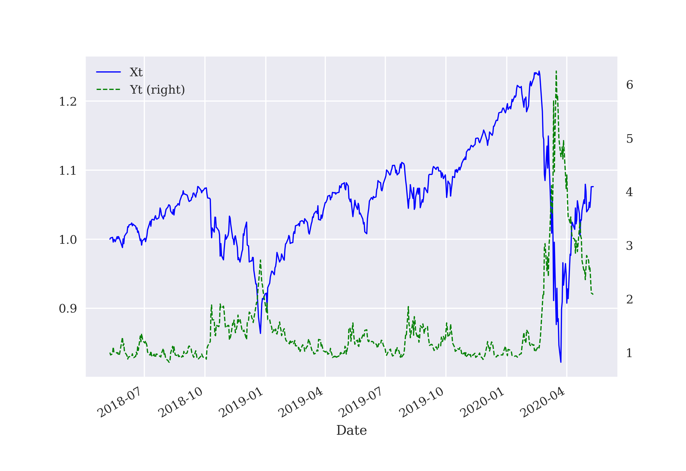
Figure 33. Normalized index levels for S&P 500 and VIX

No adjustments need to be made to the InvestingAgent class. The following code trains the agent based on the new Investing environment:

In [66]: set_seeds()

In [67]: investing = Investing(steps=days)

In [68]: agent = InvestingAgent('2AC', feature=None, n_features=5,
                              env=investing, hu=48, lr=0.0005)

In [69]: agent.xp = 3  (1)
         agent.yp = 4  (2)

In [70]: episodes = 250

In [71]: %time agent.learn(episodes)
         episode= 250 | treward=-42.749 | max=-38.6463
         CPU times: user 8min 14s, sys: 1min 38s, total: 9min 53s
         Wall time: 8min 51s

In [72]: agent.epsilon
Out[72]: 0.5348427211156283

1	Sets the index position for the first risky asset.
2	Sets the index position for the second risky asset.

The following Python code conducts several test runs. It also provides high level statistics for the allocation to the first risky asset:

In [73]: agent.env.portfolios = pd.DataFrame()

In [74]: %time agent.test(10)
         CPU times: user 37.8 s, sys: 5.39 s, total: 43.1 s
         Wall time: 35.8 s

In [75]: agent.env.portfolios['xt'].describe()
Out[75]: count   5030.000
         mean       0.433
         std        0.084
         min        0.000
         25%        0.389
         50%        0.428
         75%        0.498
         max        0.676
         Name: xt, dtype: float64

A deeper analysis of a specific test case sheds more light on the investment strategy of the agent. In the specific case chosen, the strategy keeps the allocations over the investment horizon relatively constant on average, as is illustrated in Allocation to the first risky asset. However, there are also larger re-balancings, depending on the relative performance of the two risky assets:

In [76]: n = max(agent.env.portfolios['e']) - 3

In [77]: res = agent.env.portfolios[
                 agent.env.portfolios['e'] == n].set_index('date')

In [78]: res['xt'].plot(lw=1, c='b')
         plt.ylim(res['xt'].min() - 0.1, res['xt'].max() + 0.1)
         plt.ylabel('allocation (asset 1)');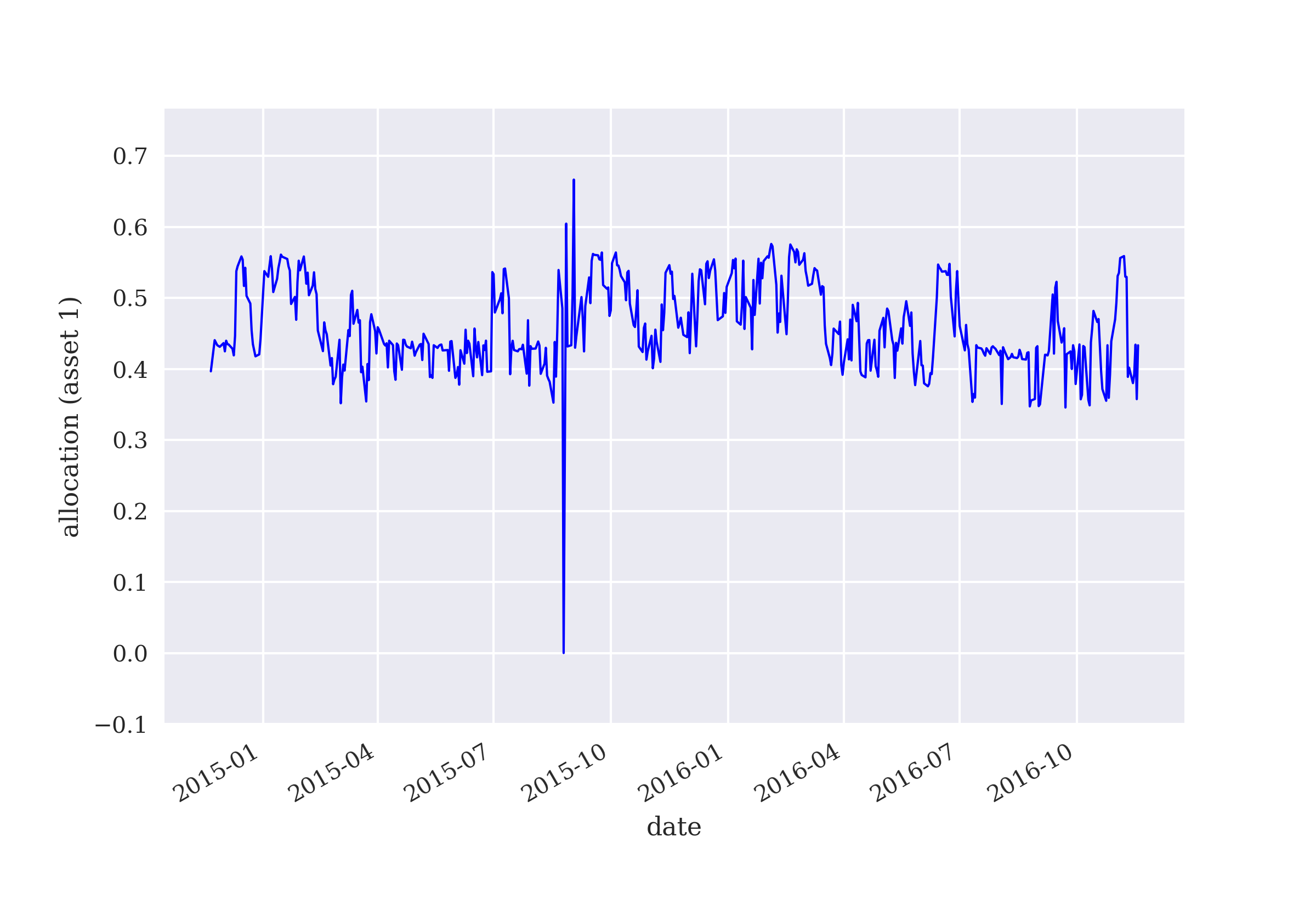

Figure 34. Allocation to the first risky asset

In the specific case chosen, the agent’s strategy does not only outperform both risky assets by a large margin, it also achieves the highest Sharpe ratio. Asset prices and portfolio value over time illustrates the performance of the agent’s strategy compared to the two risky assets:

In [79]: res[['Xt', 'Yt', 'pv']].iloc[-1]
Out[79]: Xt   1.065
         Yt   0.983
         pv   2.022
         Name: 2016-11-18 00:00:00, dtype: float64

In [80]: r = np.log(res[['Xt', 'Yt', 'pv']] /
                    res[['Xt', 'Yt', 'pv']].shift(1))

In [81]: rets = np.exp(r.mean() * 252) - 1
         rets
Out[81]: Xt    0.032
         Yt   -0.009
         pv    0.424
         dtype: float64

In [82]: stds = r.std() * math.sqrt(252)
         stds
Out[82]: Xt   0.146
         Yt   1.338
         pv   0.670
         dtype: float64

In [83]: rets / stds
Out[83]: Xt    0.221
         Yt   -0.006
         pv    0.633
         dtype: float64

In [84]: res[['Xt', 'Yt', 'pv']].plot(
             title='PORTFOLIO VALUE',
             style=['g--', 'b:', 'r-'],
             lw=1, grid=True)
         plt.ylabel('value');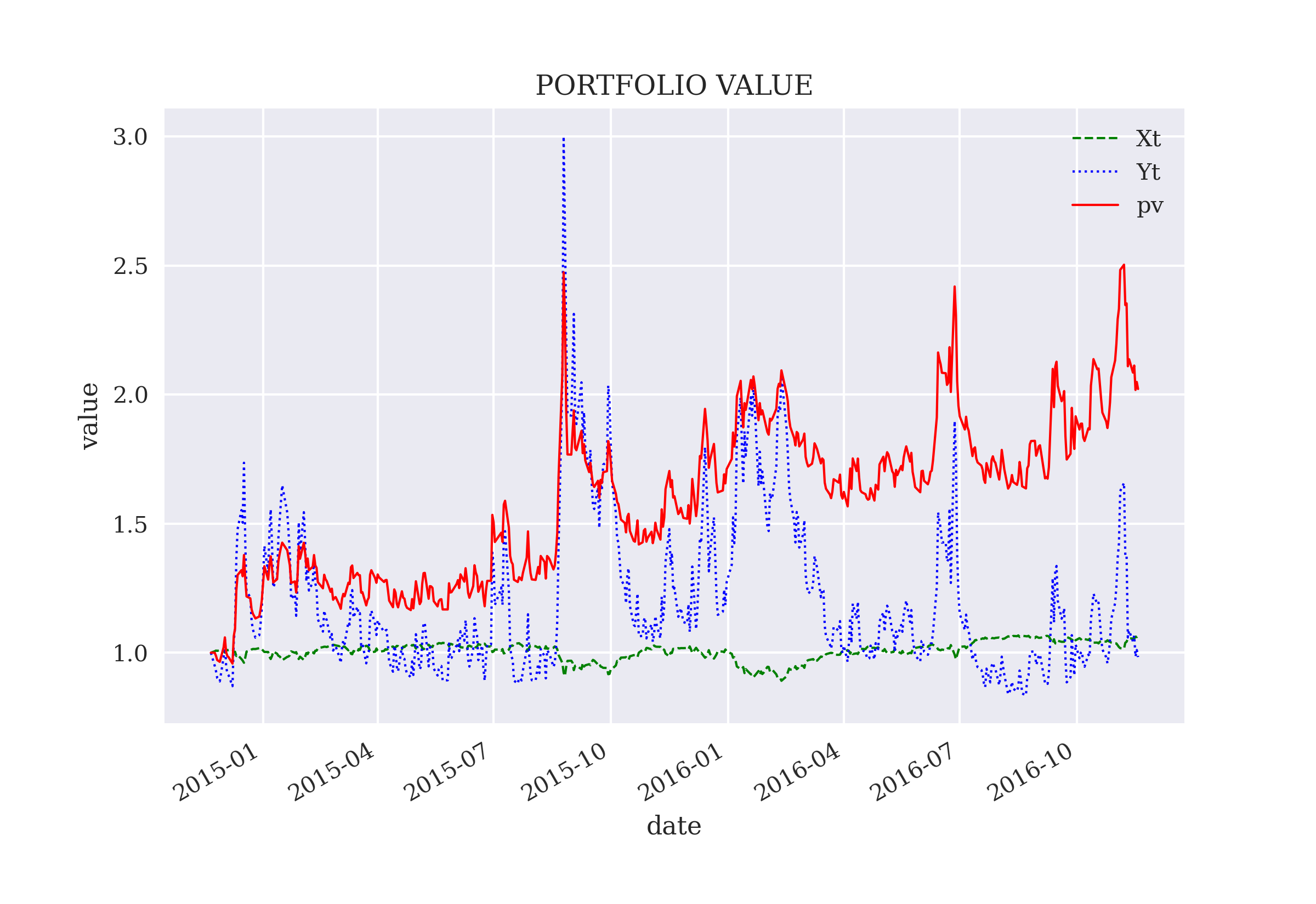

Figure 35. Asset prices and portfolio value over time

For all test runs, the agent’s strategy outperforms both assets over the investment horizon:

In [85]: values = agent.env.portfolios.groupby('e')[
                 ['Xt', 'Yt', 'pv_new']].last()
         values.tail()
Out[85]:        Xt    Yt  pv_new
         e
         256 1.285 1.067   1.998
         257 1.065 0.983   1.971
         258 1.301 1.138   2.558
         259 1.196 1.103   2.175
         260 1.389 1.373   2.672

In [86]: values.mean()
Out[86]: Xt       1.233
         Yt       1.077
         pv_new   2.187
         dtype: float64

In [87]: ((values['pv_new'] > values['Xt']) &
          (values['pv_new'] > values['Yt'])).value_counts()
Out[87]: True    10
         Name: count, dtype: int64

8.3. Three-Asset Case

This section addresses an investment case with three risky assets. It is a case that is already analyzed by Markowitz (1952) in a static setting, that is, with two points in time only. As before, the setup in this section is a dynamic one based on historical data from which a random, contiguous sample is selected for each episode during training and testing.

The code for this section is presented in the form of a Python script in Three-Asset Code. In a sense, the code presents a summary of the code of the previous two sections. It also includes the necessary adjustments, of course, to reflect the additional asset. Based on this code, a further generalization to n > 3 assets is not too difficult.

Given the Python code in Three-Asset Code, the setup is efficient. One just needs to execute the script:

In [1]: %run assetallocation.py

For the instantiation of the Investing environment, three symbols are required. Random, contiguous price samples for the three risky assets shows a randomly chosen sub-set of the time series data for the symbols.

In [2]: days = 2 * 252

In [3]: random.seed(100)

In [4]: # 1 = X, 2 = Y, 3 = Z
        investing = Investing('.SPX', '.VIX', 'XAU=', steps=days)

In [5]: investing.data.plot(lw=1, style=['g--', 'b:', 'm-.'])
        plt.ylabel('price');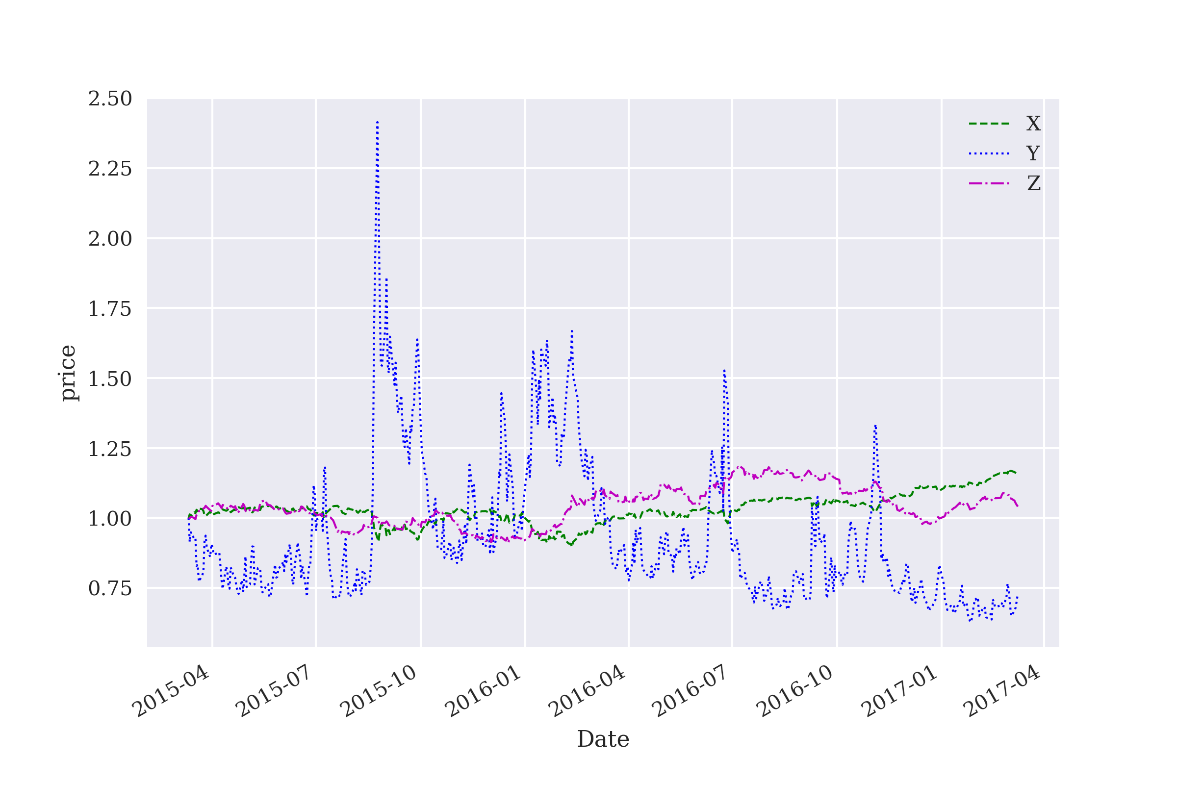

Figure 36. Random, contiguous price samples for the three risky assets

The following Python code implements the training phase for the InvestingAgent:

In [6]: random.seed(100)
        np.random.seed(100)
        tf.random.set_seed(100)

In [7]: agent = InvestingAgent('3AC', feature=None, n_features=6,
                             env=investing, hu=128, lr=0.00025)

In [8]: episodes = 64

In [9]: %time agent.learn(episodes)
        episode=  64 | treward=  2.201 | max=  7.745
        CPU times: user 1min 7s, sys: 9.85 s, total: 1min 17s
        Wall time: 1min 19s

In [10]: agent.epsilon
Out[10]: 0.8519730927255319

For the test runs, the InvestingAgent achieves an average final portfolio value that lies well above the final value of any of the three risky assets. This is achieved by allocating the largest portion on average to the first asset and the lowest portion on average to the third asset.

In [11]: agent.env.portfolios = pd.DataFrame()

In [12]: %time agent.test(10)
         episode=10 | total reward=8.24
         CPU times: user 52.9 s, sys: 7.34 s, total: 1min
         Wall time: 53.1 s

In [13]: agent.env.portfolios.groupby('e')[
             ['xt', 'yt', 'zt']].mean().mean()
Out[13]: xt    0.572418
         yt    0.341007
         zt    0.086576
         dtype: float64

In [14]: agent.env.portfolios.groupby('e')[
             ['Xt', 'Yt', 'Zt', 'pv']].last().mean()
Out[14]: Xt    1.184271
         Yt    1.303997
         Zt    1.219622
         pv    2.927294
         dtype: float64

The method to derive the optimal action of the InvestingAgent class includes a penalty term for derivations from the previous portfolio position. This avoids relatively large dynamic position adjustments as Dynamic allocation to the three risky assets visualizes for a specific test run. However, while the agent starts with an almost equally weighted portfolio, it quickly adjusts the allocations depending on the evolution of the asset prices:

In [15]: def get_r(n):
             r = agent.env.portfolios[
                 agent.env.portfolios['e'] == n
                 ].set_index('date')
             return r

In [16]: n = min(agent.env.portfolios['e']) + 1
         n
Out[16]: 66

In [17]: r = get_r(n)

In [18]: r[['xt', 'yt', 'zt']].mean()
Out[18]: xt    0.518429
         yt    0.375992
         zt    0.105579
         dtype: float64

In [19]: r[['xt', 'yt', 'zt']].std()
Out[19]: xt    0.089908
         yt    0.127021
         zt    0.147788
         dtype: float64

In [20]: r[['xt', 'yt', 'zt']].plot(
             title='ALLOCATIONS [%]',
             style=['g--', 'b:', 'm-.'],
             lw=1, grid=True)
         plt.ylabel('allocation');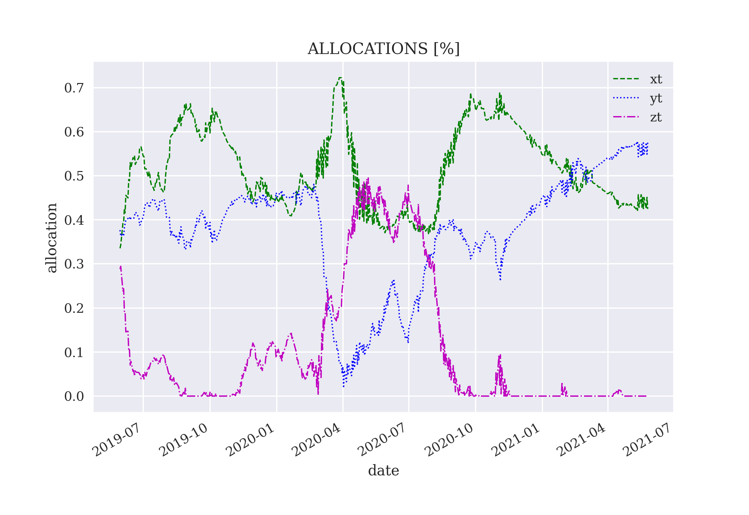

Figure 37. Dynamic allocation to the three risky assets

For that test run, Performance of the agent’s portfolio in comparison shows the performance over time of the agent’s portfolio compared to the three risky assets. In this case, the agent’s dynamic investment strategy not only achieves the highest return, it also achieves the highest Sharpe ratio by a large margin.

In [21]: cols = ['Xt', 'Yt', 'Zt', 'pv']

In [22]: sub = r[cols]

In [23]: rets = sub.iloc[-1] / sub.iloc[0] - 1
         rets
Out[23]: Xt    0.504887
         Yt    0.052514
         Zt    0.484728
         pv    2.670451
         dtype: float64

In [24]: stds = sub.pct_change().std() * math.sqrt(252)
         stds
Out[24]: Xt    0.261492
         Yt    1.475499
         Zt    0.167226
         pv    0.529418
         dtype: float64

In [25]: rets / stds
Out[25]: Xt    1.930792
         Yt    0.035591
         Zt    2.898632
         pv    5.044123
         dtype: float64

In [26]: sub.plot(style=['g--', 'b:', 'm-.', 'r-'], lw=1)
         plt.ylabel('value');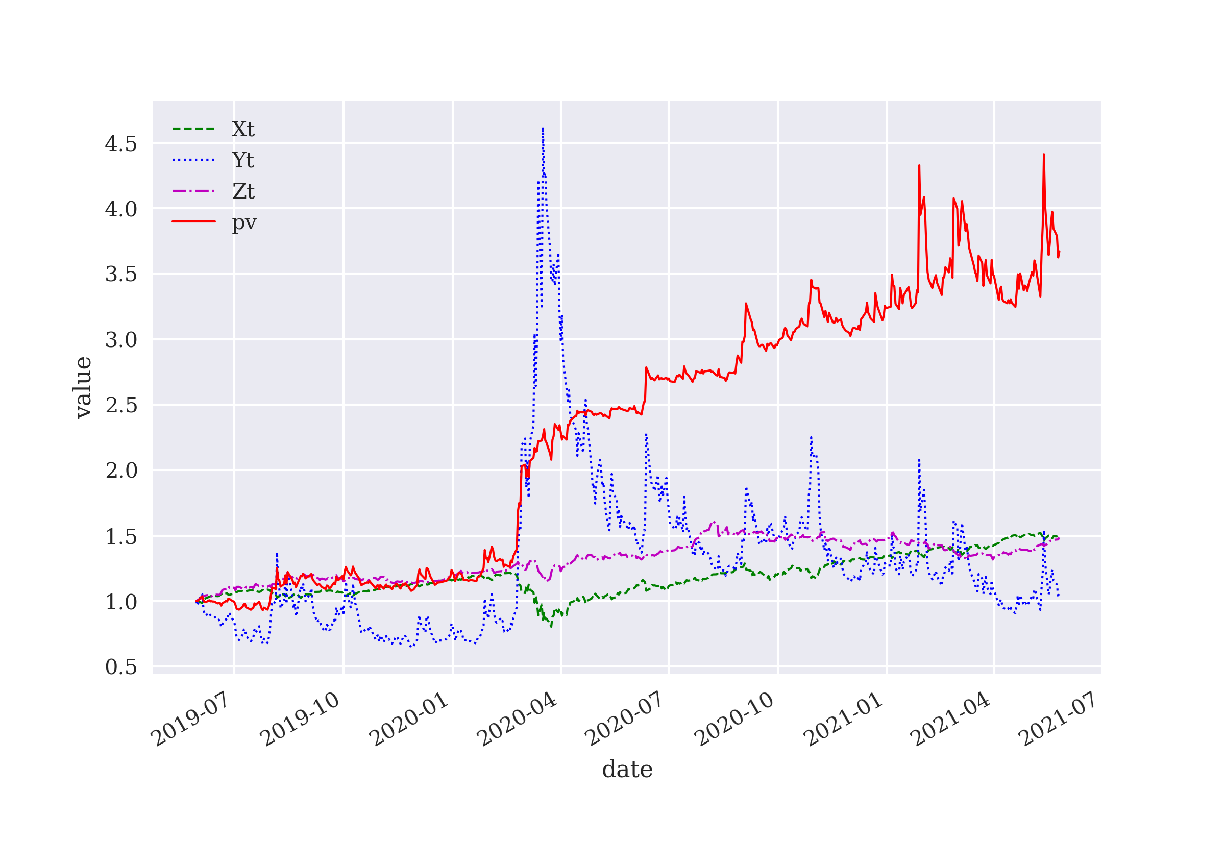

Figure 38. Performance of the agent’s portfolio in comparison

The reward that the agent receives is based on the Sharpe ratio that it realizes step-by-step. This rewards a higher return and penalizes higher risk. Therefore, it is also interesting to look at the realized Sharpe ratios during all the test runs in comparison to the three risky assets. The numbers speak a clear language. The agent’s allocations achieve on average a much higher Sharpe ration than each individual asset:

In [27]: sharpe = pd.DataFrame()

In [28]: def calculate_sr():
             for n in set(investing.portfolios['e']):
                 r = get_r(n)
                 sub = r[cols]
                 rets = sub.iloc[-1] / sub.iloc[0] - 1
                 stds = sub.pct_change().std() * math.sqrt(252)
                 sharpe[n] = rets / stds

In [29]: calculate_sr()

In [30]: sharpe.round(2)
Out[30]:       65    66    67    68    69    70    71    72    73    74
         Xt  1.69  1.93 -0.01  0.41  0.16  1.34  0.30  1.31  1.52  0.53
         Yt  0.29  0.04 -0.13 -0.05 -0.14  0.31  0.76 -0.11  0.21  0.80
         Zt  2.78  2.90  0.86 -0.21  0.51  0.71  2.13  1.12  1.19  3.24
         pv  6.55  5.04  2.08  1.11  2.32  3.67  7.09  2.80  3.76  7.84

In [31]: sharpe.mean(axis=1)
Out[31]: Xt    0.917560
         Yt    0.197753
         Zt    1.523657
         pv    4.225037
         dtype: float64

The observed outperformance on average also translates into outperformances for every single test run. The agent achieves for every test run a higher Sharpe ratio than any of the three risky assets:

In [32]: ((sharpe.loc['pv'] > sharpe.loc['Xt']) &
          (sharpe.loc['pv'] > sharpe.loc['Yt']) &
          (sharpe.loc['pv'] > sharpe.loc['Zt'])).value_counts()
Out[32]: True    10
         Name: count, dtype: int64

Simplistic Modelling

The approaches and implementations in this chapter are admittedly pretty simplistic. For example, the state of the environment contains only the current prices of the assets to be invested in, their price differences maybe, and their current allocations. In that sense, a Markov process for the evolution of the risky assets' prices is assumed — only the current price is relevant for the future evolution and not the price history.

As another example, two or three assets are also too few for real-world applications in general. However, the investment cases presented are canonical and important examples in the financial literature about portfolio theory.

Furthermore, the analysis in this chapter assumes zero transaction costs. As several of the figures in this chapter illustrate, the dynamic re-allocations of the agent are happening basically every trading day, which would lead to pretty high transaction costs. This type of assumption is, however, in line with the analysis in Dynamic Hedging.

All of this can, of course, be adjusted, enriched, and enhanced in a relatively straightforward manner.

8.4. Equally Weighted Portfolio

It is well known that an equally weighted portfolio is a hard benchmark to crack for most active and dynamic asset allocation approaches. This holds true in the case of the previous section as well. The following Python code replaces the .opt_action() method by a simple one that only returns the equal weights vector $\left( \frac{1}{3}, \frac{1}{3}, \frac{1}{3} \right)$. The results with regard to the Sharpe ratio are remarkably good on average when compared to the individual assets. For the ten test runs, the equally weighted portfolio beats the best risky asset six times. The most simple type of diversification seems to have indeed good characteristics without leveraging any type of information or analysis.

In [33]: agent.opt_action = lambda state: np.ones(3) / 3

In [34]: agent.env.portfolios = pd.DataFrame()

In [35]: %time agent.test(10)
         episode=10 | total reward=4.75
         CPU times: user 1.98 s, sys: 47.7 ms, total: 2.03 s
         Wall time: 3.53 s

In [36]: sharpe = pd.DataFrame()

In [37]: calculate_sr()

In [38]: sharpe.round(2)
Out[38]:       75    76    77    78    79    80    81    82    83    84
         Xt  1.35  0.41  2.73  1.10  0.38  3.46  1.35  0.81  0.61  1.84
         Yt  0.06  0.20 -0.08  0.62 -0.02 -0.18  0.06 -0.05  0.75 -0.16
         Zt  1.23 -0.44  0.37  1.52 -0.16 -0.87  1.23 -0.72  4.86  1.30
         pv  1.67  1.52  1.32  2.52  1.25  0.96  1.67  1.27  3.77  1.76

In [39]: sharpe.mean(axis=1)
Out[39]: Xt    1.402960
         Yt    0.121449
         Zt    0.830933
         pv    1.769955
         dtype: float64

In [40]: ((sharpe.loc['pv'] > sharpe.loc['Xt']) &
          (sharpe.loc['pv'] > sharpe.loc['Yt']) &
          (sharpe.loc['pv'] > sharpe.loc['Zt'])).value_counts()
Out[40]: True     6
         False    4
         Name: count, dtype: int64

8.5. Conclusions

Dynamic asset allocation is another financial problem that can be attacked with methods from RL and DQL. This chapter covers three different, canonical use cases:

One risky and one risk-less asset,
Two risky assets, and
Three risky assets.

A popular investment strategy is the 60/40 investment portfolio that puts 60% in risky assets, such as equity indices, and 40% in less risky assets, such as government or corporate bonds. The examples in Two-Fund Separation almost exactly recover this type of strategy in that the risky allocation of the InvestingAgent often closely hovers around 60%. Nevertheless, the agent also reacts quickly when the risky assets value drops below a certain threshold.

Two-Asset Case replaces the risk-less asset by a another risky asset. The assets chosen, the S&P 500 stock index and its volatility index VIX, are known to be highly negatively correlated. This in general implies that diversification pays off handsomely. The results for the agent’s dynamic asset allocation strategy are in general a higher absolute return and a higher Sharpe ratio.

The three-asset case as presented in Three-Asset Case is a generalization of the two-asset case. This investment case, in its static form, is already analyzed in the seminal paper on modern portfolio theory by Markowitz (1952). The dynamic strategies of the agent are able to outperform any of the three individual assets in terms of the Sharpe ratio for seven out of the ten test runs implemented.

8.6. References

Books and articles cited in this chapter:

Black, Fischer and Myron Scholes (1973): “The Pricing of Options and Corporate Liabilities.” Journal of Political Economy, Vol. 81, No. 3, 638–659.
Chisholm, Denise (2023): “Three Key Catalysts for the 60/40 Strategy.” Commentary, Fidelity Investments.
Copeland, Thomas E., Fred J. Weston, and Kuldeep Shastri (2005): Financial Theory and Corporate Policy. 4th ed., Pearson Addison Wesley, Boston et al.
Markowitz, Harry (1952): “Portfolio Selection.” Journal of Finance, Vol. 7, No. 1, 77-91.
Merton, Robert (1969): “Lifetime Portfolio Selection under Uncertainty: The Continuous-Time Case.” The Review of Economics and Statistics, Vol. 51, No. 3, 247-257.
Merton, Robert (1973): “Theory of Rational Option Pricing.” Bell Journal of Economics and Management Science, Vol. 4, No. 1, 141–183.
Poundstone, William (2010): Fortune’s Formula. Hill and Wang, New York.
The Economist (2023): “The $100trn battle for the world’s wealthiest people.” 05. September 2023.

8.7. Three-Asset Code

The following Python code provides the two main classes Investing and InvestingAgent for the three-asset investment case.

#
# Investing Environment and Agent
# Three Asset Case
#
# (c) Dr. Yves J. Hilpisch
# Reinforcement Learning for Finance
#

import os
import math
import random
import numpy as np
import pandas as pd
from scipy import stats
from pylab import plt, mpl
from scipy.optimize import minimize

from dqlagent import *

plt.style.use('seaborn-v0_8')
mpl.rcParams['figure.dpi'] = 300
mpl.rcParams['savefig.dpi'] = 300
mpl.rcParams['font.family'] = 'serif'
np.set_printoptions(suppress=True)

opt = keras.optimizers.legacy.Adam

os.environ['PYTHONHASHSEED'] = '0'
os.environ['TF_CPP_MIN_LOG_LEVEL'] = '3'


class observation_space:
    def __init__(self, n):
        self.shape = (n,)


class action_space:
    def __init__(self, n):
        self.n = n
    def seed(self, seed):
        random.seed(seed)
    def sample(self):
        rn = np.random.random(3)
        return rn / rn.sum()


class Investing:
    def __init__(self, asset_one, asset_two, asset_three,
                 steps=252, amount=1):
        self.asset_one = asset_one
        self.asset_two = asset_two
        self.asset_three = asset_three
        self.steps = steps
        self.initial_balance = amount
        self.portfolio_value = amount
        self.portfolio_value_new = amount
        self.observation_space = observation_space(4)
        self.osn = self.observation_space.shape[0]
        self.action_space = action_space(3)
        self.retrieved = 0
        self._generate_data()
        self.portfolios = pd.DataFrame()
        self.episode = 0

    def _generate_data(self):
        if self.retrieved:
            pass
        else:
            url = 'https://certificate.tpq.io/rl4finance.csv'
            self.raw = pd.read_csv(url, index_col=0, parse_dates=True).dropna()
            self.retrieved
        self.data = pd.DataFrame()
        self.data['X'] = self.raw[self.asset_one]
        self.data['Y'] = self.raw[self.asset_two]
        self.data['Z'] = self.raw[self.asset_three]
        s = random.randint(self.steps, len(self.data))
        self.data = self.data.iloc[s-self.steps:s]
        self.data = self.data / self.data.iloc[0]

    def _get_state(self):
        Xt = self.data['X'].iloc[self.bar]
        Yt = self.data['Y'].iloc[self.bar]
        Zt = self.data['Z'].iloc[self.bar]
        date = self.data.index[self.bar]
        return np.array(
            [Xt, Yt, Zt, self.xt, self.yt, self.zt]
            ), {'date': date}
        
    def seed(self, seed=None):
        if seed is not None:
            random.seed(seed)
            
    def reset(self):
        self.xt = 0
        self.yt = 0
        self.zt = 0
        self.bar = 0
        self.treward = 0
        self.portfolio_value = self.initial_balance
        self.portfolio_value_new = self.initial_balance
        self.episode += 1
        self._generate_data()
        self.state, info = self._get_state()
        return self.state, info

    def add_results(self, pl):
        df = pd.DataFrame({
                   'e': self.episode, 'date': self.date, 
                   'xt': self.xt, 'yt': self.yt, 'zt': self.zt,
                   'pv': self.portfolio_value, 'pv_new': self.portfolio_value_new,
                   'p&l[$]': pl, 'p&l[%]': pl / self.portfolio_value_new * 100,
                   'Xt': self.state[0],  'Yt': self.state[1], 'Zt': self.state[2],
                   'Xt_new': self.new_state[0],  'Yt_new': self.new_state[1],
                   'Zt_new': self.new_state[2],
                          }, index=[0])
        self.portfolios = pd.concat((self.portfolios, df), ignore_index=True)
        
    def step(self, action):
        self.bar += 1
        self.new_state, info = self._get_state()
        self.date = info['date']
        if self.bar == 1:
            self.xt = action[0]
            self.yt = action[1]
            self.zt = action[2]
            pl = 0.
            reward = 0.
            self.add_results(pl)
        else:
            self.portfolio_value_new = (
                self.xt * self.portfolio_value * self.new_state[0] / self.state[0] +
                self.yt * self.portfolio_value * self.new_state[1] / self.state[1] +
                self.zt * self.portfolio_value * self.new_state[2] / self.state[2]
            )
            pl = self.portfolio_value_new - self.portfolio_value
            self.xt = action[0]
            self.yt = action[1]
            self.zt = action[2]
            self.add_results(pl)
            ret = self.portfolios['p&l[%]'].iloc[-1] / 100 * 252
            vol = self.portfolios['p&l[%]'].rolling(
                20, min_periods=1).std().iloc[-1] * math.sqrt(252)
            sharpe = ret / vol
            reward = sharpe
            self.portfolio_value = self.portfolio_value_new
        if self.bar == len(self.data) - 1:
            done = True
        else:
            done = False
        self.state = self.new_state
        return self.state, reward, done, False, {}
        

class InvestingAgent(DQLAgent):
    def _create_model(self, hu, lr):
        self.model = Sequential()
        self.model.add(Dense(hu, input_dim=self.n_features,
                        activation='relu'))
        self.model.add(Dense(hu, activation='relu'))
        self.model.add(Dense(1, activation='linear'))
        self.model.compile(loss='mse',
                optimizer=opt(learning_rate=lr))
        
    def opt_action(self, state):
        bnds = 3 * [(0, 1)]
        cons = [{'type': 'eq', 'fun': lambda x: x.sum() - 1}]
        def f(state, x):
            s = state.copy()
            s[0, 3] = x[0]
            s[0, 4] = x[1]
            s[0, 5] = x[2]
            pen = np.mean((state[0, 3:] - x) ** 2)
            return self.model.predict(s)[0, 0] - pen
        try:
            state = self._reshape(state)
            self.action = minimize(lambda x: -f(state, x),
                                   3 * [1 / 3],
                                   bounds=bnds,
                                   constraints=cons,
                                   options={
                                       'eps': 1e-4,
                                        },
                                   method='SLSQP'
                                  )['x']
        except:
            print(state)
        return self.action
        
    def act(self, state):
        if random.random() <= self.epsilon:
            return self.env.action_space.sample()
        action = self.opt_action(state)
        return action

    def replay(self):
        batch = random.sample(self.memory, self.batch_size)
        for state, action, next_state, reward, done in batch:
            target = reward
            if not done:
                ns = next_state.copy()
                action = self.opt_action(ns)
                ns[0, 3:] = action
                target += self.gamma * self.model.predict(ns)[0, 0]
            self.model.fit(state, np.array([target]), epochs=1,
                           verbose=False)
        if self.epsilon > self.epsilon_min:
            self.epsilon *= self.epsilon_decay

    def test(self, episodes, verbose=True):
        for e in range(1, episodes + 1):
            state, _ = self.env.reset()
            state = self._reshape(state)
            treward = 0
            for _ in range(1, len(self.env.data) + 1):
                action = self.opt_action(state)
                state, reward, done, trunc, _ = self.env.step(action)
                state = self._reshape(state)
                treward += reward
                if done:
                    templ = f'episode={e} | '
                    templ += f'total reward={treward:4.2f}'
                    if verbose:
                        print(templ, end='\r')
                    break
        print()

9. Optimal Execution

Since the 2007-2008 crisis, Quantitative Finance has changed a lot. In addition to the classical topics of derivatives pricing, portfolio management, and risk management, a swath of new subfields has emerged, and a new generation of researchers is passionate about systemic risk, market impact modeling, counterparty risk, high-frequency trading, optimal execution, etc.

— Guéant (2016)

Traditional finance theory often assumes that the actions of agents do not have any impact on markets or prices because they are “so small” as compared to the group of all market participants. All applications in Financial Applications so far fall also into that category: no matter what the action of the agent is, the prices of the traded assets are not influenced.

In reality, however, trading relatively small quantities of shares of a stock can, in fact, have an impact on their prices. This is even more so the case for large buy-side institutions, such as hedge funds, or large intermediaries, such as investment banks, who often need to trade large blocks of shares.

The trade-off that traders face in such situations is between a fast execution that might have a large impact on prices or a slower execution that has a smaller impact on prices but that leads to price risks due to the “natural” fluctuations in market prices.

By assumption, this trade-off is not present in Algorithmic Trading, Dynamic Hedging, and Dynamic Asset Allocation. The typical assumption in models like the one of Black-Scholes-Merton (1973) discussed in Dynamic Hedging is one of perfectly liquid markets or infinitesimally small agents. If, in that model, markets are imperfectly liquid and the dynamically hedging agent has a non-negligible market share, then the prices of European put and call options are not as derived by Black-Scholes-Merton but rather higher due to the effects that dynamic hedging has on the market price of the underlying.^[26]

This chapter addresses the optimal execution of large block trades over a number of trading days. Such a task fits well into the general framework of dynamic programming. The chapter relies on the model by Almgren and Chriss (1999) — or AC99 for short. The AC model is one of the first to account for different types of costs associated with the liquidation of large positions in a stock or multiple stocks. The chapter proceeds as follows: The Model describes the model itself and provides a closed form solution for the case in which the single traded asset follows a random walk. Model Implementation implements the model in Python and illustrates the impact of different combinations for the main model parameters. Execution Environment develops an environment for the sequential execution of block trades on the basis of the AC99 model. Execution Agent discusses the execution agent that learns to optimally execute large block trades in the AC99 model.

9.1. The Model

Traditional finance theory assumes that the value of a position in a stock at time $t$ is given by the number of shares, $X$, multiplied by the price of a share at that time, $S_t$. However, in practice the liquidation of a large position in a stock might be impossible due to a lack of market liquidity or might significantly lower prices to attract more buyers.^[27] Therefore, the value under liquidation of a large position in a stock often is significantly lower than $X \cdot S_t$.

More realistically, the AC99 model assumes that the liquidation of a large block of shares is executed over a number of trading days, $t=0, 1, 2, \dots, T$, with only partial quantities of $x_0, x_1, \dots, x_T$ liquidated per day with $\sum_t x_t = X$. In its basic form, the AC99 model assumes that the single stock follows a random walk, $dS_t = \sigma dZ_t$, where $Z_t$ is a Brownian motion and $S_0$ is fixed.^[28]

Furthermore, the model assumes three sources of execution costs associated with such a liquidation. The first is the permanent impact with impact factor $\gamma$. It is linear in the number of shares traded and is defined as:

\[\text{Permanent Impact} = \gamma \sum_{t=1}^T x_i\]

The second is the temporary impact with temporary impact factor $\eta$. With $\Delta t$ being the time interval between two trading days, the temporary impact is given by:

\[\text{Temporary Impact} = \eta \sum_{t=1}^T \left( \frac{x_t}{\Delta t} \right)^2 \Delta t\]

The third is the execution risk, where $\lambda$ is the risk aversion factor of the executing agent and $\sigma$ is the volatility factor of the stock:

\[\text{Execution Risk} = \lambda \sigma^2 \sum_{t=1}^T \left( \frac{X - \sum_{i=1}^{t-1} x_i}{\Delta t} \right)^2 \Delta t\]

The total execution costs are given as:

\[\begin{array}{} \text{TEC} &=& \text{Permanent Impact} + \text{Temporary Impact} + \text{Execution Risk} \\ &=& \gamma \sum_{t=1}^T x_t + \eta \sum_{t=1}^T \left( \frac{x_t}{\Delta t} \right)^2 \Delta t + \lambda \sigma^2 \sum_{t=1}^T \left( \frac{X - \sum_{i=1}^{t-1} x_i}{\Delta t} \right)^2 \Delta t \end{array}\]

The dynamic optimization problem in the AC99 model therefore becomes:

\[\underset{ x_t, t \in \{0, 1, \dots , T\} }{ \min } \text{TEC}\]

subject to

\[\sum_{t=0}^T x_t = X\]

It can be shown, using calculus of variations or dynamic programming, that in the basic form of the AC99 model, the optimal trading trajectory satisfies the following differential equation:

\[\frac{d^2 x}{dt^2} - \frac{\lambda \sigma^2}{\eta} x = 0\]

It can be further shown that a general solution to this differential equation is given by:

\[x_t = A \cosh(\kappa(T - t)) + B \sinh(\kappa(T - t))\]

Here, $\kappa = \sqrt{\frac{\lambda \sigma^2}{\eta}}$ and $A, B$ are constants determined by the boundary conditions.

Applying the boundary conditions $x_0 = X$ and $x_T = 0$, one obtains the following specific solution for the optimal quantity $x^*_t$ to be liquidated until $t$:

\[x^*_t = \frac{X \sinh(\kappa(T - t))}{\sinh(\kappa T)}\]

For more details on the AC99 model and enhancements of it, refer to Almgren and Chriss (1999), Almgren and Chriss (2000), and Guéant (2016).

From a practical point of view, the estimation of the main model parameters is obviously of paramount importance. The following empirical methods can be used for the estimation:

$\gamma$: The permanent market impact parameter can be estimated through a regression of stock price changes against the volume of trades that caused the changes. More specific market micro-structure models, such as the one by Kyle (1985) and its successors, can also be used.
$\eta$: The temporary market impact parameter can be estimated through the analysis of intraday or high-frequency data to measure the impact of single trades on the market prices. In addition, order book dynamics can be analyzed to gain more insights in the role of different order book depths in this context.
$\lambda$: Utility-based analyses can be used to estimate the risk aversion factor. One can also backtest and calibrate the AC99 model to find a value for $\lambda$ that brings the model’s predictions best in line with actual trading data.

In the following section, two different parameter combinations are assumed for the model. The only parameter that is varied is the risk aversion factor $\lambda$ because it influences the optimal liquidation strategy significantly.

9.2. Model Implementation

With the background from The Model, the following implementation with its variable definitions and naming conventions should be straightforward to understand. First, the imports:

In [1]: import math
        import random
        import numpy as np
        import pandas as pd
        from pylab import plt, mpl

from pprint import pprint
In [2]: plt.style.use('seaborn-v0_8')
        mpl.rcParams['figure.dpi'] = 300
        mpl.rcParams['savefig.dpi'] = 300
        mpl.rcParams['font.family'] = 'serif'
        np.set_printoptions(suppress=True)

Second, the initialization:

In [3]: class AlmgrenChriss:
            def __init__(self, T, N, S0, sigma, X, gamma, eta, lamb):
                self.T = T
                self.N = N
                self.dt = T / N
                self.S0 = S0
                self.sigma = sigma
                self.X = X
                self.gamma = gamma
                self.eta = eta
                self.lamb = lamb

Third, the optimal execution policy and trading trajectory. As Optimal execution for high and low risk aversion ($\lambda$) illustrates, a higher risk aversion leads to an initially faster execution policy than a lower risk aversion. With high $\lambda$, the agent first liquidates larger quantities from the total position and then reduces the quantity over time. In the case with low $\lambda$, the agent trades almost equal quantities per trading day. In the end, however, both strategies completely liquidate the original position.

In [4]: class AlmgrenChriss(AlmgrenChriss):
            def optimal_execution(self):
                kappa = np.sqrt(self.lamb * self.sigma ** 2 / self.eta)
                t = np.linspace(0, self.T, self.N + 1)
                xt_sum = (self.X * np.sinh(kappa * (self.T - t)) /
                          np.sinh(kappa * self.T))
                xt = -np.diff(xt_sum, prepend=0)
                xt[0] = 0
                return t, xt

In [5]: T = 10  (1)
        N = 10  (2)
        S0 = 1  (3)
        sigma = 0.15  (4)
        X = 1  (5)
        gamma = 0.1  (6)
        eta = 0.1  (7)
        lamb_high = 0.2  (8)
        lamb_low = 0.0001  (8)

In [6]: ac = AlmgrenChriss(T, N, S0, sigma, X, gamma, eta, lamb_high)

In [7]: t, xth = ac.optimal_execution()

In [8]: t
Out[8]: array([ 0.,  1.,  2.,  3.,  4.,  5.,  6.,  7.,  8.,  9., 10.])

In [9]: xth.round(3)  (9)
Out[9]: array([0.   , 0.197, 0.161, 0.132, 0.109, 0.091, 0.077, 0.067, 0.059,
               0.054, 0.052])

In [10]: ac.lamb = lamb_low

In [11]: t, xtl = ac.optimal_execution()
         xtl.round(3)  (10)
Out[11]: array([0. , 0.1, 0.1, 0.1, 0.1, 0.1, 0.1, 0.1, 0.1, 0.1, 0.1])

In [12]: plt.plot(t, ac.X - xth.cumsum(), 'r', lw=1,
                  label='high $\\lambda$ (position)')
         plt.plot(t, xth, 'rs', markersize=4,
                  label='high $\\lambda$ (trade)')
         plt.plot(t, ac.X- xtl.cumsum(), 'b--', lw=1,
                  label='low $\\lambda$ (position)')
         plt.plot(t, xtl, 'bo', markersize=4,
                  label='low $\\lambda$ (trade)')
         plt.ylabel('trading day')
         plt.ylabel('shares (normalized to 1)')
         plt.legend();

1	The time horizon in trading days.
2	The number of trading days.
3	The initial stock price (normalized to 1).
4	The volatility of the stock price (quite high).
5	The total position to be liquidated (normalized to 1).
6	The permanent impact factor.
7	The temporary impact factor.
8	The high and low risk aversion factors for the agent.
9	The trading trajectory for high risk aversion.
10	The trading trajectory for low risk aversion.

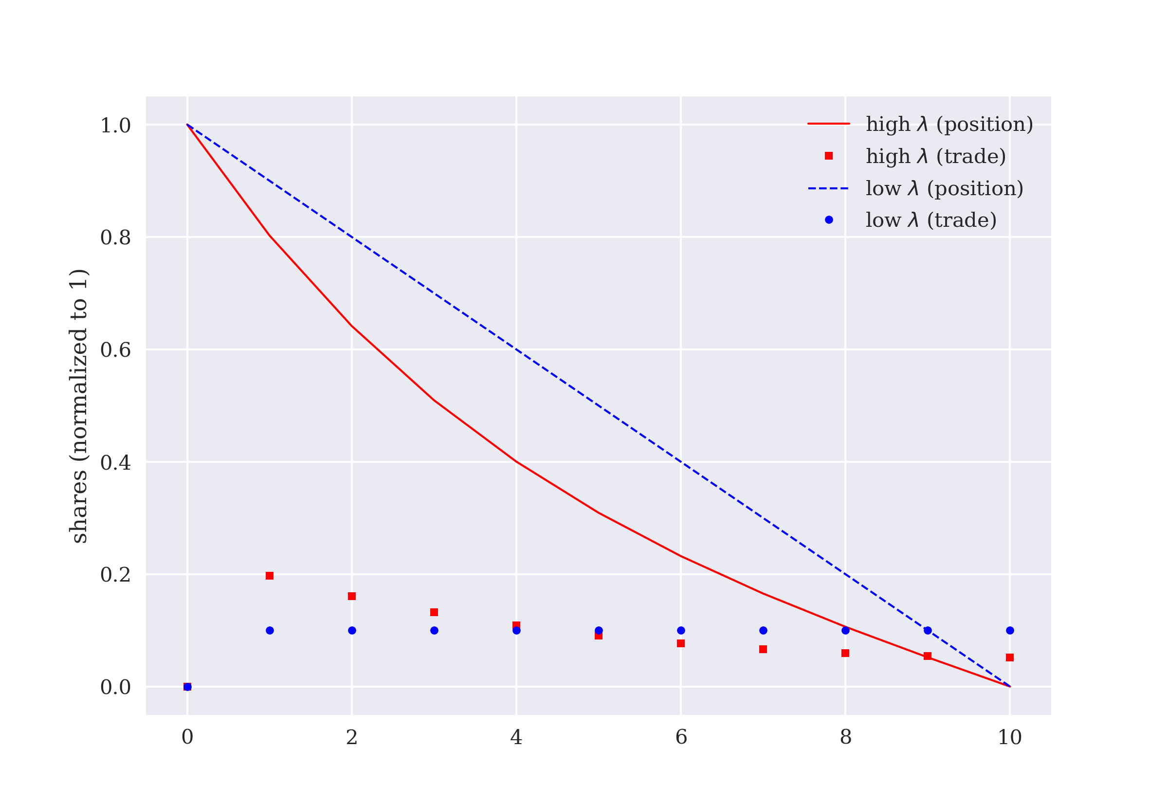
Figure 39. Optimal execution for high and low risk aversion ($\lambda$)

Fourth, the simulation of the stock price process. To see meaningful effects throughout, the volatility factor has been chosen quite high given the implementation of the Monte Carlo simulation with regard to the random numbers drawn.

In [13]: from numpy.random import default_rng

In [14]: class AlmgrenChriss(AlmgrenChriss):
             def simulate_stock_price(self, xt, seed=None):
                 rng = default_rng(seed=seed)
                 S = np.zeros(self.N + 1)  (1)
                 S[0] = self.S0  (1)
                 P = np.zeros(self.N + 1)  (2)
                 P[0] = self.S0  (2)
                 for t in range(1, self.N + 1):
                     dZ = rng.normal(0, np.sqrt(self.dt))
                     S[t] = S[t - 1] + sigma * dZ  (1)
                     P[t] = S[t] - self.gamma * xt[:t + 1].sum()  (2)
                 return S, P

1	Simulated stock price path.
2	Adjusted stock price path for permanent impact.

The following examples illustrate the impact of high and low risk aversion on the stock price over time. With high $\lambda$, the stock is more impacted early on than with low $\lambda$. This is reasonable because high risk aversion leads, by comparison, to larger quantities sold early on. Adjusted stock price paths for high and low risk aversion ($\lambda$) illustrates the effects visually.

In [15]: ac = AlmgrenChriss(T, N, S0, sigma, X, gamma, eta, lamb_high)

In [16]: t, xth = ac.optimal_execution()

In [17]: xth.round(2)
Out[17]: array([0.  , 0.2 , 0.16, 0.13, 0.11, 0.09, 0.08, 0.07, 0.06, 0.05,
          0.05])

In [18]: seed = 250

In [19]: S, Ph = ac.simulate_stock_price(xth, seed=seed)

In [20]: ac.lamb = lamb_low

In [21]: t, xtl = ac.optimal_execution()

In [22]: xtl.round(2)
Out[22]: array([0. , 0.1, 0.1, 0.1, 0.1, 0.1, 0.1, 0.1, 0.1, 0.1, 0.1])

In [23]: S, Pl = ac.simulate_stock_price(xtl, seed=seed)

In [24]: plt.plot(t, S, 'b', lw=1, label='simulated stock price path')
         plt.plot(t, Ph, 'r--', lw=1, label='adjusted path (high $\\lambda$)')
         plt.plot(t, Pl, 'g:', lw=1, label='adjusted path (low $\\lambda)')
         plt.xlabel('trading day')
         plt.ylabel('stock price (normalized to 1)')
         plt.legend();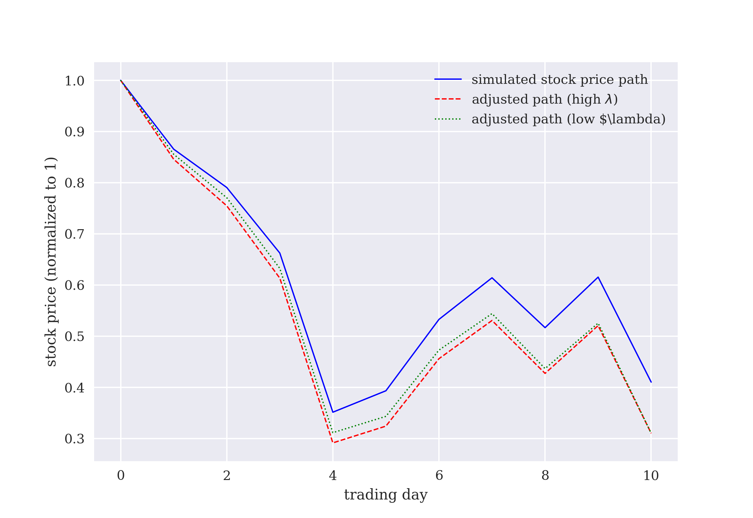

Figure 40. Adjusted stock price paths for high and low risk aversion ($\lambda$)

Parameter Values

The parameter values chosen in this section are relative extreme, such as for the volatility of the stock price — given that the time horizon is a only few days. This is done to generate noticeable effects from the simulation and when changing, for example, the risk aversion parameter. In practical applications, all parameters should be carefully calibrated to market realities.

The final method added to the AlmgrenChriss class is for the calculation of the single cost factors and the total execution cost. As the numbers demonstrate, high risk aversion leads to high total execution costs while low risk aversion leads to basically reduced costs in all categories. The permanent impact costs are almost comparable. The temporary impact costs are much higher in the high $\lambda$ case because of the quadratic term in the calculation formula. The largest difference however is observed in the execution risk. That number is much higher due to the much higher $\lambda$ factor in the calculation formula.

In [25]: class AlmgrenChriss(AlmgrenChriss):
             def calculate_costs(self, xt):
                 temporary_cost = np.sum(self.eta *
                             (xt / self.dt) ** 2 * self.dt)
                 permanent_cost = np.sum(self.gamma * np.cumsum(xt) * xt)
                 execution_risk = self.lamb * self.sigma ** 2 * np.sum(
                     (np.cumsum(xt[::-1])[::-1] / self.dt) ** 2 * self.dt)
                 TEC = temporary_cost + permanent_cost + execution_risk
                 return temporary_cost, permanent_cost, execution_risk, TEC

In [26]: ac = AlmgrenChriss(T, N, S0, sigma, X, gamma, eta, lamb_high)

In [27]: t, xth = ac.optimal_execution()

In [28]: tc, pc, er, TEC = ac.calculate_costs(xth)

In [29]: print(f'lambda = {ac.lamb}')
         print(f'temporary cost = {tc:7.4f}')
         print(f'permanent cost = {pc:7.4f}')
         print(f'execution risk = {er:7.4f}')
         print(f'total ex. cost = {TEC:7.4f}')  (1)
         lambda = 0.2
         temporary cost =  0.0122
         permanent cost =  0.0561
         execution risk =  0.0165
         total ex. cost =  0.0848

In [30]: ac.lamb = lamb_low

In [31]: t, xtl = ac.optimal_execution()

In [32]: tc, pc, er, TEC = ac.calculate_costs(xtl)

In [33]: print(f'lambda = {ac.lamb}')
         print(f'temporary cost = {tc:7.4f}')
         print(f'permanent cost = {pc:7.4f}')
         print(f'execution risk = {er:7.4f}')
         print(f'total ex. cost = {TEC:7.4f}')  (2)
         lambda = 0.0001
         temporary cost =  0.0100
         permanent cost =  0.0550
         execution risk =  0.0000
         total ex. cost =  0.0650

1	Total execution costs for low risk aversion ($\lambda$).
2	Total execution costs for high risk aversion ($\lambda$).

A somewhat extreme analogy might further illustrate the role of risk aversion in the AC99 model. Suppose you are in a building in which a small fire breaks out. If you are extremely risk averse, you run out of the building and call the fire fighters. In the meantime, the fire spreads further in the building and damages more and more furniture as time passes. If you are not that risk averse, you stay calm, look for a fire extinguisher, try to contain the fire, and reduce potential damage in the building. In the meantime, you can still call the fire fighters who will fully get the fire under control once they arrive. The damage is much smaller in the second case than in the first one, but at the risk of getting injured or even worse.

A similar story can be told about a store that is in need of liquidity. The store manager can decide to dump all products at a discount of 80% on a single day (“fire sale”) or they can decide on a longer sale period at average discounts of 40%.

In the AC99 model, as a rule of thumb, the quantities to be traded on the single trading days are equal in the case of a risk-neutral agent, that is, an agent which is not risk averse at all. On the other hand, a risk averse agent wants to get rid of larger quantities early on but then at (much) higher execution costs. *

The next section implements an execution environment based on the AC99 model.

9.3. Execution Environment

For the Execution class, the parameters and attributes are the same as for the AlmgrenChriss class with one addition for the number of episodes:

In [34]: class Execution:
             def __init__(self, T, N, S0, sigma, X, gamma, eta, lamb):
                 self.T = T
                 self.N = N
                 self.dt = T / N
                 self.S0 = S0
                 self.sigma = sigma
                 self.X = X
                 self.gamma = gamma
                 self.eta = eta
                 self.lamb = lamb
                 self.episode = 0

The state of the execution environment is given by the complete liquidation trajectory, plus the remaining shares, the time passed (in percent), and the current trade (action).

In [35]: class Execution(Execution):
             def _get_state(self):
                 s = np.array([self.X_,  (1)
                             self.bar / self.N])  (2)
                 state = np.hstack((self.xt, s))  (3)
                 return state, {}
             def reset(self):
                 self.bar = 0
                 self.treward = 0
                 self.episode += 1
                 self.X_ = self.X  (1)
                 self.xt = np.zeros(self.N + 1)  (4)
                 self.tec = pd.DataFrame(
                     {'pc': 0, 'tc': 0, 'er': 0}, index=[0])  (5)
                 return self._get_state()

1	The remaining shares.
2	The time passed (percent).
3	Full state array object.
4	The trading trajectory.
5	`DataFrame` object for cost storage.

The major task for the .step() method is the calculation and storage of the single cost components and the TEC. There is also a large penalty added to the TEC when there are shares remaining at the end of the trading period.

In [36]: class Execution(Execution):
             def step(self, action):
                 self.bar += 1
                 self.xt[self.bar] = action  (1)
                 self.X_ -= action  (2)
                 pc = np.sum(self.gamma *
                         np.cumsum(self.xt) * self.xt)  (3)
                 tc = np.sum(self.eta *
                         (self.xt / self.dt) ** 2 * self.dt)  (3)
                 er = self.lamb * self.sigma ** 2 * np.sum(
                     (np.cumsum(self.xt[::-1])[::-1] / self.dt) ** 2
                     * self.dt)  (3)
                 df = pd.DataFrame({'pc': tc, 'tc': pc, 'er': er},
                                   index=[0])  (3)
                 self.tec = pd.concat((self.tec, df))  (3)
                 cost = self.tec.diff().fillna(0).iloc[-1]  (3)
                 tec = cost.sum()  (3)
                 self.state, _ = self._get_state()
                 pen = 0
                 if self.bar < self.N:
                     if self.X_ <= 0.0001:
                         done = True
                     else:
                         done = False
                 elif self.bar == self.N:
                     pen = abs(self.X_) * 10  (4)
                     done = True
                 return self.state, -(tec + pen), done, False, {}

1	The current trade (action) is added.
2	The remaining shares are adjusted.
3	The costs are calculated and stored.
4	A penalty is added for non-liquidated shares.

The following code illustrates the interaction with the environment based on simple liquidation strategies. The agent is assumed to be almost risk neutral (low $\lambda$). The first example liquidates the position on the first trading day completely. The TEC are accordingly on their highest possible level. The second example liquidates 50% on the first trading day and 50% on the second trading day. The total liquidation costs are already much lower. The third example liquidates the position in ten equal trades which gives the minimal TEC as calculated before:

In [37]: execution = Execution(T, N, S0, sigma, X, gamma, eta, lamb_low)

In [38]: execution.reset()
         execution.step(1.0)  (1)
Out[38]: (array([0. , 1. , 0. , 0. , 0. , 0. , 0. , 0. , 0. , 0. , 0. , 0. ,
          0.1]),
          -0.2000045,
          True,
          False,
          {})

In [39]: execution.reset()
Out[39]: (array([0., 0., 0., 0., 0., 0., 0., 0., 0., 0., 0., 1., 0.]), {})

In [40]: execution.step(0.5)  (2)
Out[40]: (array([0. , 0.5, 0. , 0. , 0. , 0. , 0. , 0. , 0. , 0. , 0. , 0.5,
          0.1]),
          -0.050001125,
          False,
          False,
          {})

In [41]: execution.step(0.5)  (3)
Out[41]: (array([0. , 0.5, 0.5, 0. , 0. , 0. , 0. , 0. , 0. , 0. , 0. , 0. ,
          0.2]),
          -0.0750039375,
          True,
          False,
          {})

In [42]: execution.reset()
         cost = list()
         for i in range(10):
             cost.append(execution.step(0.1)[1])  (4)
         print(f'TEC = {sum(cost):.3f}')
         TEC = -0.065

1	Liquidates 100% on the first trading day.
2	Liquidates 50% on the first trading day …
3	… and 50% on the second trading day.
4	Liquidates 10% on each of the 10 trading days.

9.4. Random Agent

This section implements a random agent for interaction with the Execution environment. The problem at hand requires a more specialized approach than just drawing a few random numbers independently. One major requirement is that the random numbers — that is, the random trades — for the single trading days add up to one. To this end, one can use the Dirichlet distribution which is implemented in the numpy.random sub-package (see Dirichilet). It allows the drawing of multiple random numbers that by definition add up to one.

The following examples show the TEC for random liquidation trajectories for both low and high risk aversion:

In [43]: execution = Execution(T, N, S0, sigma, X, gamma, eta, lamb_low)  (1)

In [44]: rng = default_rng(seed=100)

In [45]: def gen_rn():
             alpha = np.ones(N)  (2)
             rn = rng.dirichlet(alpha)  (2)
             rn = np.insert(rn, 0, 0)  (3)
             return rn

In [46]: rn = gen_rn()
         rn  (4)
Out[46]: array([0.        , 0.15895546, 0.12542041, 0.07457818, 0.00209012,
                0.08708588, 0.02557811, 0.05065022, 0.23502973, 0.16044992,
                0.08016197])

In [47]: rn.sum()  (5)
Out[47]: 1.0000000000000002

In [48]: def execute_trades():
             for _ in range(5):
                 execution.reset()
                 rn = gen_rn()
                 for i in range(1, 11):
                     execution.step(rn[i])  (6)
                 tec = execution.tec.iloc[-1].sum()
                 print(f'TEC = {tec:.3f}')

In [49]: execute_trades()  (7)
         TEC = 0.072
         TEC = 0.078
         TEC = 0.081
         TEC = 0.071
         TEC = 0.099

In [50]: execution = Execution(T, N, S0, sigma, X, gamma, eta, lamb_high)  (8)

In [51]: execute_trades()  (9)
         TEC = 0.105
         TEC = 0.103
         TEC = 0.097
         TEC = 0.097
         TEC = 0.093

1	Execution environment with low risk aversion.
2	Draws the random, Dirichlet-distributed numbers.
3	Adds a zero as the first value.
4	A sample set of random numbers.
5	They add up to one as desired.
6	Executes the random trades.
7	The resulting TEC are higher than the minimal TEC.
8	Execution environment with high risk aversion.
9	Again, the TEC are higher than the minimal TEC.

9.5. Execution Agent

The basic setup for optimal execution seems similar to the one for dynamic hedging in Dynamic Hedging and asset allocation in Dynamic Asset Allocation. After all, the agent is supposed to choose a single floating point number per action. However, the optimal execution problem is different in that every action is bound above by the remaining shares and in that all actions over the trading period must add up to one.

The rather simple algorithmic implementation in the previous chapters does not work well in the context of this chapter. Previously, every single action was basically independent of the other actions. Here, this is not the case. The set of feasible actions and the optimal trade on the tenth trading day, say, is influenced by the actions taken on all other trading days before.

Therefore, this section introduces what is called an actor-critic algorithm for RL. While this type of algorithm shares many characteristics with DQL algorithms, they are considered to form their own category of algorithm. An actor-critic algorithm has the following major elements:

Actor or Action Policy: The actor which is represented by the action policy — which in turn is modeled as a DNN — chooses an action given a state of the environment.
Critic or Value Function: The critic, which is represented by the value function, again typically a DNN, maps a certain state to a value where higher usually means better.

In the implementation, three major steps are repeatedly executed:

The actor chooses an action given a certain state and its policy.
Based on its value function, the critic provides feedback on these actions by comparing the predicted value of the new state with the actual reward received and the estimated value of the previous state.
The actor uses the feedback to update its policy to increase the expected reward.

In this context, it is important that the feedback is primarily based on whether the actor’s action is better than to be expected or worse. The critic also updates its policy according to the observed reward and the estimated value for the new state.

Algorithmic Differences

In the previous two chapters, the DQL agents use only one policy $Q$ to map a state and an action simultaneously to a single value $(s, a) \mapsto Q(s, a)$. Changing the action changes the value, which allows for an optimization procedure to find the action that maximizes the value for the given state. Such an approach is typically called a value-based method in DQL. With the actor-critic algorithm, a separation takes place into two major elements: the action policy $A$, mapping a state to an action $s \mapsto A(s)$, and a value function $Q$, mapping a state to a value $s \mapsto Q(s)$.

The following Python code implements such an actor-critic algorithm. Overall, the implementation is still quite similar to the previous implementations of the DQL agents. First, the initialization part:

In [52]: from dqlagent import *

In [53]: random.seed(100)
         tf.random.set_seed(100)

In [54]: opt = keras.optimizers.legacy.Adam

In [55]: class ExecutionAgent(DQLAgent):
             def __init__(self, symbol, feature, n_features, env,
                          hu=24, lr=0.0001, rng='equal'):
                 self.epsilon = 1.0
                 self.epsilon_decay = 0.9975
                 self.epsilon_min = 0.1
                 self.memory = deque(maxlen=2000)
                 self.batch_size = 32
                 self.eta = 1.0
                 self.trewards = list()
                 self.max_treward = -np.inf
                 self.n_features = n_features
                 self.env = env
                 self.episodes = 0
                 self.rng = rng
                 self._generate_rn()  (1)
                 self.actor = self._create_model(hu, lr, 'sigmoid')  (2)
                 self.critic = self._create_model(hu, lr, 'linear')  (3)

1	Generates the first set of random numbers
2	Creates the DNN for the actor.
3	Created the DNN for the critic.

Second, the generation of appropriate random numbers for the random trades to be executed during exploration. The implementation makes sure that sets of random numbers are drawn that are exhibiting different characteristics:

In [56]: class ExecutionAgent(ExecutionAgent):
             def _generate_rn(self):
                 if self.rng == 'equal':
                     alpha = np.ones(self.env.N)  (1)
                 elif self.rng == 'decreasing':
                     alpha = range(self.env.N, 0, -1)   (2)
                 else:
                     alpha = rng.random(self.env.N)  (3)
                 rn = rng.dirichlet(alpha)
                 self.rn = np.insert(rn, 0, 0)

1	Array with equal values.
2	Array with decreasing values.
3	Array with purely random values.

Third, the creation of the DNNs for the actor and the critic. The implementation allows you to choose the appropriate activation function for the two DNNs. For the actor, the sigmoid function is appropriate because the actor is supposed to choose an action between zero and one. For the critic, the linear function is appropriate:

In [57]: class ExecutionAgent(ExecutionAgent):
             def _create_model(self, hu, lr, out_activation):
                 model = Sequential()
                 model.add(Dense(hu, input_dim=self.n_features,
                                 activation='relu'))
                 model.add(Dense(hu, activation='relu'))
                 model.add(Dense(1, activation=out_activation))
                 model.compile(loss='mse', optimizer=opt(learning_rate=lr))
                 return model

Fourth, the .act() method. Here, the agent is supposed to rely solely on exploration for relatively large number of episodes. This provides the agent with enough experience before relying on its action policy and value function:

In [58]: class ExecutionAgent(ExecutionAgent):
             def act(self, state):
                 if random.random() <= self.epsilon or self.episodes < 250:  (1)
                     return min(self.rn[self.f], state[0, -2])  (2)
                 else:
                     action = self.actor.predict(state)[0, 0]  (3)
                 return action

1	Independent of `self.epsilon`, the agent only explores for a larger number of episodes.
2	Random actions (trades) are clipped at the value for the remaining shares.
3	The actor chooses an optimal trade according to its policy.

Fifth, the major part that implements the actor-critic algorithm in the .replay() method:

In [59]: class ExecutionAgent(ExecutionAgent):
             def replay(self):
                 batch = random.sample(self.memory, self.batch_size)
                 for state, action, next_state, reward, done in batch:
                     target = reward
                     if not done:
                         target += self.eta * self.critic.predict(
                                 next_state)[0, 0]  (1)
                         self.critic.fit(state, np.array([target]),
                                 epochs=1, verbose=False)  (2)
                         # advantage = target - self.critic.predict(state)[0, 0]
                         self.actor.fit(state, np.array([action]),
                                 # sample_weight=np.array([advantage]),
                                 epochs=1, verbose=False)  (3)
                 if self.epsilon > self.epsilon_min:
                     self.epsilon *= self.epsilon_decay
                 self._generate_rn()  (4)

1	Adds the expected, discounted value for the next state to the reward.
2	Updates the value function of the critic.
3	Updates the action policy of the actor.
4	Generates a new set of random actions.^[29]

Finally, the .test() which shows only minor changes as compared to the ones from the previous chapters:

In [60]: class ExecutionAgent(ExecutionAgent):
             def test(self, episodes, verbose=True):
                 for e in range(1, episodes + 1):
                     state, _ = self.env.reset()
                     state = self._reshape(state)
                     treward = 0
                     for _ in range(1, self.env.N + 1):
                         action = self.actor.predict(state)[0, 0]  (1)
                         state, reward, done, trunc, _ = self.env.step(action)
                         state = self._reshape(state)
                         treward += reward
                         if done:
                             templ = f'total reward={treward:4.3f}'
                             if verbose:
                                 print(templ)
                             break
                     print(self.env.xt)

1	The actor chooses an optimal action according to its policy.

With the ExecutionAgent class completed, training of the agent can take place. First, the case for the low risk aversion factor. In that case, the agent learns the optimal strategy — that is, the liquidation of the initial position in equal trade sizes — rather quickly:

In [61]: execution = Execution(T, N, S0, sigma, X, gamma, eta, lamb_low)

In [62]: executionagent = ExecutionAgent(None, feature=None,
                             n_features=execution.N + 3,
                             env=execution, hu=64, lr=0.0001,
                             rng='equal')

In [63]: episodes = 2500

In [64]: %time executionagent.learn(episodes)
         episode=2500 | treward= -0.270 | max= -0.065
         CPU times: user 2min 38s, sys: 43 s, total: 3min 21s
         Wall time: 2min 25s

In [65]: executionagent.test(1)
         total reward=-0.912
         [0.         0.09795619 0.09197164 0.09160777 0.09103356 0.09467734
          0.09440769 0.09722784 0.08991307 0.08550413 0.07989337]

In [66]: xtl_ = execution.xt
         xtl_.sum()
Out[66]: 0.9141926020383835

Next, the case for the high risk aversion factor. In this case, the agent also learns pretty well that it is optimal to sell more shares earlier and to decrease the trade size over time:

In [67]: execution = Execution(T, N, S0, sigma, X, gamma, eta, lamb_high)

In [68]: executionagent = ExecutionAgent(None, feature=None,
                             n_features=execution.N + 3,
                             env=execution, hu=64, lr=0.0001,
                             rng='decreasing')

In [69]: %time executionagent.learn(episodes)
         episode=2500 | treward= -0.280 | max= -0.085
         CPU times: user 2min 40s, sys: 44.2 s, total: 3min 25s
         Wall time: 2min 27s

In [70]: executionagent.test(1)
         total reward=-0.199
         [0.         0.18177003 0.16303268 0.14493093 0.11896227 0.10893401
          0.08658476 0.07199006 0.05079928 0.03398583 0.02749112]

In [71]: xth_ = execution.xt
         xth_.sum()
Out[71]: 0.9884809665381908

Finally, Optimal and learned trading trajectories for high and low $\lambda$ compares the learned trading trajectories of the agent with the optimal ones. With the appropriate configuration of the random number and action generation for exploration, the agent is able to learn the optimal execution trajectories quite well. However, the agent does not match the optimal strategies perfectly for the configurations used.

In [72]: plt.plot(xtl[1:], 'b', lw=1, label='optimal for low $\lambda$')
         plt.plot(xtl_[1:], 'b:', lw=1, label='learned for low $\lambda$')
         plt.plot(xth[1:], 'r--', lw=1, label='optimal for high $\lambda$')
         plt.plot(xth_[1:], 'r-.', lw=1, label='learned for high $\lambda$')
         plt.legend();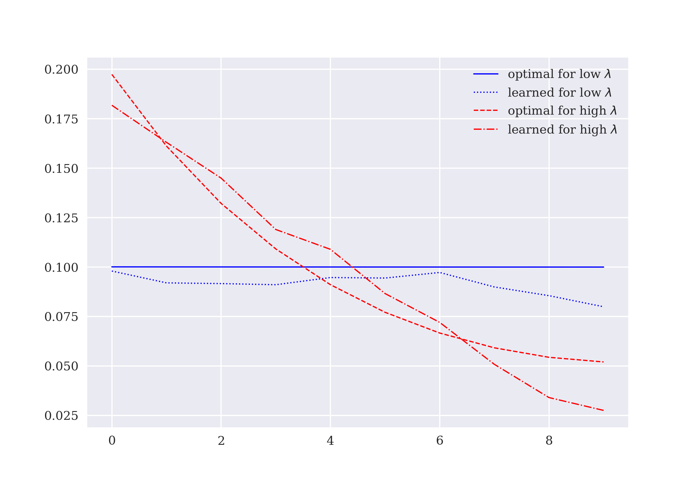

Figure 41. Optimal and learned trading trajectories for high and low $\lambda$

9.6. Conclusions

The optimal execution of large trades is an important problem both in theoretical and even more so in practical finance. In reality, even relatively small trades can move prices significantly — contrary to many financial models that assume perfectly liquid markets. Therefore, selling a large position in a stock might have a large impact on the stock price. On the other hand, distributing the liquidation over a longer period introduces market price risk, that is, the price might move unfavorably independent of the liquidation. For a risk-neutral agent that latter risk is not of particular importance. However, it is important to a risk-averse agent. The problem that arises is a dynamic optimization problem whose goal it is to minimize total transaction costs given a certain level of risk aversion.

In the AC99 model, the optimal execution policy for a risk-neutral agent therefore is characterized by equal trade sizes over the assumed number of trading days. By contrast, the optimal policy for a risk-averse agent is to sell more shares in the beginning and fewer shares later on because this reduces the risk resulting from market price changes. With appropriate priming of the execution agent in the form of different types of random numbers/actions — either decreasing on average or being more equal leveled — the agent is able to learn the optimal execution trajectories quite well.

The execution agent in this chapter is modeled based on an actor-critic algorithm. It shares some similarities with the value-based DQL agent from previous chapters. However, there are also major differences. While the DQL agents use a single network to come up with an optimal action for a given state, the actor-critic agent uses one network for the optimal action policy (actor) and one network for the value function (critic) that both interact with each other. This architecture is similar to the two networks of a GAN interacting with each other to generate synthetic data (see Generated Data). Using this algorithm, the execution agent can come up with an optimal policy that spans multiple, interrelated actions. This is in contrast to the previous problems where the actions of the agents are primarily independent of each other and the current action is not directly connected to historical or future actions.

Loosely connected vs. tightly connected actions

The financial problems considered in Algorithmic Trading through Dynamic Asset Allocation can be compared, to some extent at least, to betting on the outcomes of a repeated, biased coin-tossing game. The problem is about taking actions that over time lead to a maximum reward. But the actions taken are neither conditioned on past actions nor on future actions — just on the current state.

The optimal execution problem considered in this chapter is rather like a chess game where the current move is, at least in part, dependent on past moves and is also dependent on potential future moves. With the optimal execution problem there is the major constraint that all actions taken need to add up to the original position. This tightly connects all the actions with each other.

9.7. References

Almgren, Robert and Neil Chriss (1999): “Value under Liquidation.” Risk, December 1999, Download.
Almgren, Robert and Neil Chriss (2000): “Optimal Execution of Portfolio Transactions.” Journal of Risk, Vol. 3, 5–39.
Guéant, Olivier (2016): The Financial Mathematics of Market Liquidity. CRC Press, Boca Raton.
Hilpisch, Yves (2000): Dynamic Hedging, Positive Feedback, and General Equilibrium. Dissertation, Saarland University, Download.
Kyle, Albert (1985): “Continuous Auctions and Insider Trading.”, Econometrica, Vol. 53, No. 6, 1315–1336.

10. Concluding Remarks

Time and uncertainty are the central elements that influence financial economic behavior. It is the complexity of their interaction that provides intellectual challenge and excitement to the study of finance. To analyze the effects of this interaction properly often requires sophisticated analytical tools.

— Merton (1990)

Reinforcement learning (RL) has undoubtedly become a central and important algorithm and approach in machine learning (ML) and artificial intelligence (AI) in general. There are many different flavors of the basic algorithmic idea, an overview of which can be found in Sutton and Barto (2018). This book primarily focuses on deep Q-learning (DQL). The fundamental idea of DQL is that the agent learns an optimal action policy that assigns to each feasible state-action combination a value. The higher the value, the better an action given a certain state. The book also provides in Optimal Execution an example for a simple actor-critic algorithm. In this case, the agent has the optimal action policy separated from the value function. At the core of these algorithms are deep neural networks (DNNs) that are used to approximate optimal action policies and, in the case of actor-critic algorithms, also value functions. The Basics introduces the basics of DQL and provides first, simple applications.

Finance as a domain is characterized by limited data availability. A historical time series, say, for the price of a share of a stock, is at a certain point in time given and fixed. This is in contrast to many other domains in which data can be actively generated in volumes necessary to properly train RL algorithms. The canonical example in this context are board games. An RL algorithm can interact with an environment and play, say, millions of chess games against another engine or even against itself, thereby increasing the set of experiences in an arbitrary and theoretically almost unlimited fashion.

Data Augmentation addresses this problem and introduces approaches to enrich the available financial data through methods from Monte Carlo simulation and generative adversarial networks (GANs). The use of Monte Carlo simulation has a long tradition in finance, dating back to the 1970s. Many sub-domains of finance have benefited from this flexible and powerful numerical method, such as derivatives analytics and risk management. GANs on the other hand are a rather recent innovation that allow the generation of synthetic financial data sets that share statistical characteristics with real financial data sets in a way that they become indistinguishable from a statistical point of view. GANs also rely on DNNs at their core.

Financial Applications applies DQL to important dynamic optimization problems in finance: algorithmic trading, dynamic hedging of options, and dynamic asset allocation. DQL in the context of algorithmic trading is simplified to a context where the agent only needs to decide whether to go long a financial instrument or short. In other words, the agent has only two actions to choose from. Dynamic hedging and dynamic asset allocation, on the other hand, are optimal control problems where the agent has in principle an unlimited set of feasible actions during each step. Therefore, additional optimization procedures are generally required to come up with optimal actions.

DQL takes into account by construction the immediate reward of an action and the discounted, delayed reward of an optimal future action. By the Bellmann principle, this ensures that the action policy over time leads to an approximately optimal outcome. The example in Optimal Execution is somewhat special in that all actions are tightly connected through a constraint which is not the case in the other applications. Therefore, the actor-critic algorithm is introduced in this context because it can handle such problems often better than a standard DQL approach.

The overall approach in this book is a practical one. This means that theory is only presented at a minimal level, or even omitted altogether. This also means that the implementations are kept concise and simple to be able to focus on the key issues and algorithmic aspects. However, this also implies that there are many opportunities to make the implementations more realistic, that is, closer to financial reality and more sophisticated on the side of the agents. The hope is that readers can take the provided implementations as starting points and frameworks and add their own ideas and improvements.

With regard to the applications, the environments presented in the book do not leverage all approaches for data augmentation as presented in Data Augmentation in all settings. For example, GANs are not used for the applications part but rather more simple approaches such as fixed historical data or MCS. However, it is straightforward to replace the data generating parts of the different environments by alternative approaches or to come up even with completely different environments. Furthermore, the MCS parts of the environments generally use only simple benchmark models such as geometric Brownian motion for the simulation. More sophisticated and realistic models, such as jump diffusions or stochastic volatility models, could also be used easily instead. In addition, the environments assume “perfect” markets in several respects. For example, transaction costs are neglected and perfect market liquidity is assumed in general. In this regard, Optimal Execution is again the exception in that execution costs and market impact are modeled explicitly.

On the other hand, agents could also be implemented in a more powerful way. The presented implementations generally rely on pretty basic parts, such as for the optimal policy DNNs. The same holds true for the modeling of the state which primarily defines the interaction between the environment and the agent. The presented implementations generate a pretty simple, parsimonious state object with only a few variables. Adjusting both the environments and the agents in this regard is also quite straightforward and will often lead to improved performances of the agent.

Dynamic optimization problems have a long tradition in finance and play an important role in many areas. The book by Merton (1990), for example, provides a collection of early work on the topic in the form of continuous-time models. RL, DQL, and similar algorithms are an enrichment of the tool set already available to financial academics and practitioners alike. In many instances, RL allows the application to and solution of dynamic optimization problems in finance that other methods might not be able to solve. Therefore, it is to be expected that RL will play an increasingly important role in the future in financial education and research as well as in real-world applications.

10.1. References

Sutton, Richard and Andrew Barto (2018): Reinforcement Learning: An Introduction. 2nd ed., The MIT Press, Cambridge and London.
Merton, Robert (1990): Continuous-Time Finance. Oxford University Press, New York.

Author Biography

Dr. Yves J. Hilpisch is founder and CEO of The Python Quants, a group focusing on the use of open source technologies for financial data science, artificial intelligence, algorithmic trading, computational finance, and asset management. He is also founder and CEO of The AI Machine, a company focused on AI-powered algorithmic trading via a proprietary strategy execution platform.

He is also the author of the following books:

Financial Theory with Python (O’Reilly, 2021),
Artificial Intelligence in Finance (O’Reilly, 2020),
Python for Algorithmic Trading (O’Reilly, 2020),
Python for Finance (2nd ed., O’Reilly, 2018),
Listed Volatility and Variance Derivatives (Wiley, 2017), and
Derivatives Analytics with Python (Wiley, 2015).

Yves is Adjunct Professor for Computational Finance and lectures on Reinforcement Learning for Algorithmic Trading at the CQF Program. He is also the director of the first online training program leading to a Certificate in Python for Finance.

Yves wrote the financial analytics library DX Analytics and organizes meetups, conferences, and bootcamps about Python for quantitative finance and algorithmic trading in London, Frankfurt, Berlin, Paris, and New York. He has given keynote speeches at technology conferences in the United States, Europe, and Asia.

1. Utility maximization is an economic principle that describes the process by which agents choose the best available option to achieve the highest level of satisfaction or utility given their preferences, constraints (such as income or budget), and the available alternatives.

2. Modern psychology is rather a discipline focused on university students in particular than on human beings in general. For example, Hanel and Vione (2016) conclude: “In summary, our results indicate that generalizing from students to the general public can be problematic …, as students vary mostly randomly from the general public.”

3. For a comprehensive overview of Bayesian methods in finance see Rachev et al. (2008).

4. The book by Goodfellow et al. (2016) provides a comprehensive treatment of deep neural networks.

5. See, for example, the seminal works by Watkins (1989) and Watkins and Dayan (1992).

6. See the Wikipedia article for a detailed history of this console.

7. Public interest in this achievement is, for example, reflected in the more than 34 million views (as of November 2023) of the YouTube documentary about AlphaGo.

8. The Gymnasium project is a fork of the original Gym project by OpenAI whose support and maintenance have stopped.

9. This, of course, depends on the board position at hand. There are differences between opening, middle, and end games.

10. See the blog post by DeepMind.

11. The repetition rule, for example, prevents the possibility of an infinite chess game. A player can claim a draw if a certain position is repeated at least three times.

12. The exposition follows roughly Sundaram (1996, ch. 11).

13. deque objects are similar to list objects but have a maximum number of elements only. Once it is reached and a new element is added, the first element is dropped. In that sense, it implements a “first in, first out” queue. In the context of modeling the memory of a DQL agent, the deque object mimics a human brain that remembers more recent experiences better than older ones. The approach also prevents the usage of old experiences, having been made based on a probably worse policy, to be used for replay.

14. This is a technical requirement of TensorFlow when updating DNNs based on a single sample only.

15. For the definition of different types of AI, see, for example, Hilpisch (2020, ch. 2).

16. For more details on Monte Carlo simulation with Python, see Chapter 12 of Hilpisch (2018).

17. The careful observer will notice that the three processes do not start exactly at one. This is due to the fact that the initial value gets “lost” after the calculation of the log returns and the cleaning up of the DataFrame object.

18. For details, numerical techniques, and Python code examples in the context of financial model calibration see Hilpisch (2015).

19. The KS test dates back to the seminal paper by Kolmogorov already published in 1933.

20. Hilpisch (2015) provides details for the calibration of stochastic models for Monte Carlo simulation in the context of option pricing and hedging.

21. The pandas-ta package, for example, offers an efficient way of adding typical financial indicators (features) to a given financial time series.

22. Many fast-growing technology companies also have a history of not paying any dividends, for example.

23. Given the zero risk of the riskless asset, its Sharpe ratio is not defined (infinite). For that reason, the Sharpe ratio cannot be used as a reward. The agent would learn to primarily (exclusively) invest in the riskless asset to ensure large (infinite) rewards.

24. For more details and example calculations based on Python code, see Hilpisch (2017, ch. 4). The examples in that book use the EURO STOXX stock index instead of the S&P 500 and the VSTOXX volatility index instead of the VIX.

25. In a more general setting, a penalty could also result from transaction costs, market impact, or other market microstructure elements.

26. See Hilpisch (2001) for more details on dynamic hedging in imperfectly liquid markets, resulting positive feedback and volatility effects, and their impact on option prices.

27. Other negative effects on the price might result from the negative signal that the liquidation of a position by a large, strategic investor has.

28. Contrary to the original assumption in AC99, the process is assumed to be drift-less. This seems justified given that only a relatively small number of trading days is usually assumed.

29. This is done in this place only for convenience. It prevents the adjustment of the rather long .learn() method as inherited from the DQLAgent class.

Reinforcement Learning for Finance

Copyright

Preface

Why this Book?

Target Audience

Overview of the Book

The Basics

1. Learning through Interaction

1.1. Bayesian Learning

1.1.1. Tossing a Biased Coin

1.1.2. Rolling a Biased Die

1.1.3. Bayesian Updating

1.2. Reinforcement Learning

1.2.1. Major Breakthroughs

1.2.2. Major Building Blocks

1.3. Deep Q-Learning

1.4. Conclusions

1.5. References

2. Deep Q-Learning

2.1. Decision Problems

2.2. Dynamic Programming

2.3. Q-Learning

2.4. CartPole as an Example

2.4.1. The Game Environment

2.4.2. A Random Agent

2.4.3. The DQL Agent

2.5. Q-Learning vs. Supervised Learning

2.6. Conclusions

2.7. References

3. Financial Q-Learning

3.1. Finance Environment

3.2. DQL Agent

3.3. Where the Analogy Fails

3.3.1. Limited Data

3.3.2. No Impact

3.4. Conclusions

3.5. References

Data Augmentation

4. Simulated Data

4.1. Noisy Time Series Data

4.2. Simulated Time Series Data

4.3. Conclusions

4.4. References

4.5. DQLAgent Python Class

5. Generated Data

5.1. Simple Example

5.2. Financial Example

5.3. Kolmogorov-Smirnov Test

5.4. Conclusions

5.5. References

Financial Applications

6. Algorithmic Trading

6.1. Prediction Game Revisited

6.2. Trading Environment

6.3. Trading Agent

6.4. Conclusions

6.5. References

6.6. Finance Environment

6.7. DQLAgent Class

6.8. Simulation Environment

7. Dynamic Hedging

7.1. Delta Hedging

7.2. Hedging Environment

7.3. Hedging Agent

7.4. Conclusions

7.5. References

7.6. BSM (1973) Formula

8. Dynamic Asset Allocation

8.1. Two-Fund Separation

8.2. Two-Asset Case

8.3. Three-Asset Case

8.4. Equally Weighted Portfolio

8.5. Conclusions

8.6. References

8.7. Three-Asset Code

9. Optimal Execution

9.1. The Model

9.2. Model Implementation

9.3. Execution Environment

9.4. Random Agent

4.5. `DQLAgent` Python Class